从零实现 LLM Inference：074. Multiprocess Serving 极致优化：Ablation / 稳定性 / 拓扑绑核 / Async Streaming / Profiling

在 071 里我把 roseinfer 从单进程拆成了 API process + engine process。tail 确实稳了，但拆完以后很快就会碰到一个现实问题：

多进程不是“画张架构图就结束”，它会带来一堆很真实的工程税。
线程池、绑核、IPC、loop 公平性、streaming 形态，任何一个点没抠对，性能就会漏气。

这篇我就干一件事：把这堆工程税压到我愿意长期背着的水平——默认配置就是最强；每个点都有开关；能做论文式 ablation；并且能用 profile 把结论讲清楚。

---

目标

我对 multiprocess serving 的要求其实非常苛刻：

1) 性能：MP baseline（全开）在 roseinfer variants 里应该是最优；至少不能出现“关掉某个优化反而更快”的反直觉。
2) 稳定：benchmark 能跑不算数，profile stage 偶发 crash 才是线上真正会炸的那种。
3) 可解释：每个优化点都有 option，ablation 像论文一样能复现；profile 文件位置固定、读法清晰。

对标对象我就盯三个：vLLM / SGLang / TensorRT-LLM。

---

业界复盘：他们为什么 multi-process 还能这么快？

我这次刻意把视角从“attention 算子”挪到“系统工程税”，因为 multiprocess 真正拖性能的往往就是这些。

1) 线程池：多进程 + 默认线程数 = 直接 CPU 过载

vLLM 在 multiprocess executor 里直接把 OMP_NUM_THREADS 这类东西压住，注释写得很直白：多进程默认线程数会造成 CPU contention（源码：vllm/v1/executor/multiproc_executor.py 的 set_multiprocessing_worker_envs）。

SGLang 的 GPU worker 也会在加载权重前 torch.set_num_threads(1)，理由同样是 “reduce thread conflicts”（源码：python/sglang/srt/model_executor/model_runner.py）。

结论：多进程场景下，默认线程数几乎总是负收益。

2) 输入预算：别把 scheduler loop 的 decode 给饿死

SGLang 的 scheduler 收请求时有 max_recv_per_poll 上限，达到就 break（源码：python/sglang/srt/managers/scheduler.py）。直觉很简单：极端负载下输入洪峰会吞掉一整轮 loop 时间，decode 被饿死，tail 直接爆炸。

结论：scheduler loop 必须给 decode 留预算。

3) 绑核：别“数学正确但拓扑错误”

这点 vLLM/SGLang 没把策略写死给你看，但它们都给了暗示：CPU 要当资源规划，而不是交给 OS 随缘。SGLang 甚至会给 GPU 进程设置 affinity（源码：python/sglang/srt/utils/common.py）。

我自己的坑是：混合架构（P-core/E-core）上，“把可用 CPU list 一分为二”很容易把 engine pin 到慢核，做成纯负优化（下面会详细讲）。

4) Streaming：默认就是 async

这个坑特别“线上”：Starlette/FastAPI 的 StreamingResponse 如果给 sync generator，会把 generator 丢线程池跑，本质就是 一个 stream 一条线程。vLLM/SGLang 的 OpenAI server 默认姿势都是 async streaming——它们不一定显式告诉你“别这么干”，但默认实现已经把坑绕开了。

---

我们的 root cause：为什么 071 的 multiprocess 还不够“极致”？

把 multiprocess 相比 in-proc 多出来的成本拆开看，基本就五类：

1) CPU 竞争：API+engine 都跑 PyTorch/tokenizer/detok，默认线程池把 CPU 打爆；
2) IPC 工程税：token 事件在热路径上分配 dict/list，再 pickle/queue；
3) loop 不公平：输入 drain 太狠会饿死 decode；
4) 绑核翻车：auto split 把 engine pin 到慢核 / 拆开 SMT siblings；
5) 服务边界瓶颈：StreamingResponse 的线程海把 tail 拖坏（甚至饿 GPU）。

另外还有一个“必须补作业”的点：profile stage 偶发 crash。这类 crash 线上一定会以更恶心的方式炸出来，不把它收敛掉，我不相信任何性能结论。

---

设计总览：API/Engine 两进程 + 热路径减肥

整体拓扑还是 071 的边界（API process + engine process），但这次把热路径上每一坨“杂物”都抠了一遍：

graph LR
  C[Client] -->|HTTP/SSE| API[API Process]
  API -->|Cmd: add/cancel/profile| IPC1[IPC cmd]
  IPC1 --> ENG[Engine Process]
  ENG -->|Events: token/finish| IPC2[IPC evt]
  IPC2 --> API
  API --> C
  subgraph "Hot Path"
    API
    IPC1
    ENG
    IPC2
  end

原则很简单：engine loop 里不做没必要的 Python 分配；API 侧不搞线程海；CPU 资源要规划；profile 要能复现。

---

一组默认按“正收益”打开的 MP 优化

这里我统一用论文式标记：

• -xxx：默认打开的正收益特性，ablation 是关掉它；
• +yyy：默认关闭的风险/负收益项，ablation 是打开它。

1) -thr cap：每个进程的 PyTorch/OMP 线程池都 cap 到 1，默认开

做法就是 vLLM/SGLang 那套：engine/API 两边都把 torch.set_num_threads(1) / torch.set_num_interop_threads(1)，并配套 OMP_NUM_THREADS=1 / MKL_NUM_THREADS=1。

目标不是“让单次更快”，而是 避免多进程 CPU 竞争把 tail 拖烂。

2) -affinity：topology-aware 自动绑核，默认开

我一开始的 auto split 是典型“数学正确”：把 sched_getaffinity() 的 CPU list 平分。
问题是：混合架构（以 i9-13900K 这种为代表）上，CPU id 和核快慢很可能相关；你把 engine 分到尾巴，很可能就是 E-core。

所以我现在的策略是按 physical core 分，而不是按 cpu id 分：

1) 读取 /sys/devices/system/cpu/cpu*/topology/thread_siblings_list 做 core 分组；
2) 优先把 SMT group（通常是 P-core） 分给 engine；
3) 不把同一个 physical core 的 SMT siblings 拆给两个进程；
4) 小 CPU 份额（容器只给 0-15 这类）时保证 engine 至少拿一半，否则 engine loop 会被饿死。

graph TB
  subgraph "CPU affinity set"
    P[SMT groups (often P-cores)<br/>(0,1) (2,3) ...]
    E[solo groups (often E-cores)<br/>(16) (17) ...]
  end
  P -->|prefer| ENG[engine process]
  E -->|spill| API[API process]
  ENG -->|leave enough budget| API

实现落在 rosellm/roseinfer/server.py（_cpu_core_groups() / _auto_split_cpu_affinity()）。

3) -cmd budg：输入处理预算，默认 mp_max_recv_per_iter=64

对应 SGLang 的 max_recv_per_poll：每轮最多收 N 个 cmd，剩下留给下一轮，保证 decode 不会被输入洪峰饿死。

4) pipe bytes + -flat evts：事件拍平 + 走 send_bytes/recv_bytes，默认开

目标是把 token 事件从“Python 对象海”变成“可 memcpy 的扁平数据”：

• 旧：dict[int, list[int]] / list[finished]（大量对象）
• 新：array('I') 形式的 (rid, token_id) pairs + finished_ids
• IPC 默认用 multiprocessing.Connection.send_bytes/recv_bytes，避免 multiprocessing.Queue 的 pickle/feeder thread 开销。

+queue ipc 作为对照项保留（默认关）。

5) -batch send / -fill tgt：减少 IPC 调用次数、避免碎 batch，默认开

这两个点都是纯工程：让 API->engine 的 cmd 发送更“块状”，让 engine 侧每轮更接近填满（而不是被碎片化请求打成小 batch）。

6) Offline 特有：-fast cnt 默认开，+stream tok 默认关

offline throughput 默认是 finish-only：不需要 streaming token，只要最终 output token 数。

如果你还每 step 更新 token_count dict，本质是在用“在线粒度”做“离线统计”，纯浪费 CPU。
所以 -fast cnt 的快路径是：request finished 时一次性取 scheduler.get_step_count(rid) 写最终统计。

+stream tok 则是故意把离线也打开 token event（作为对照，默认关）。

为什么 -fast cnt 一关就暴跌？

这个点我一开始也没想到会这么“夸张”，后来把代码摊开看就很清楚了：它不是那种“微调一下，+1%”的优化，而是把一坨完全没必要的 Python 热路径删掉了。

我们 offline 的 MP 路径默认是 finish-only（mp_finish_only=True）：engine 不往外发 token stream，只在请求结束时回一个 “这个请求一共生成了多少 token”。然后 benchmark 脚本用这个 count 去算 tok/s。

问题在于：你怎么得到这个 count？

• 朴素做法（+slow cnt，也就是把 -fast cnt 关掉）：
  • engine 进程自己维护一个 token_counts: dict[rid, cnt]；
  • 每一次 decode step 都会拿到 step_tokens: dict[rid, token_id]；
  • 然后在 Python 里对每个 rid 做一次 token_counts[rid] += 1；
  • 请求 finished 时，把 token_counts[rid] 发回去。

伪代码大概就是这样：

for step in range(T):
    step_tokens = scheduler.step()  # dict[rid -> token]
    for rid in step_tokens:
        token_counts[rid] += 1       # Python dict get/set 热路径

这在 “小模型 + 高吞吐” 的 offline 场景里非常致命：gpt2 在 4070 上 decode 得太快了，你很容易把瓶颈从 GPU 直接挪到 CPU。于是你会看到一个非常真实的现象：

GPU 其实能跑得更快，但你在 CPU 上为了“统计一个数”付出了 20%+ 的时间。

而 -fast cnt 的核心思想就是一句话：别重复记账。

scheduler 作为生成逻辑的一部分，本来就必须维护 “一个请求已经生成了多少步/多少 token”：

• 要判断 max_new_tokens 什么时候到；
• 要做 stop_on_eos；
• 要处理 prefix cache / overlap schedule 的一些边界。

所以我直接复用这个内部计数：请求 finished 时调用 scheduler.get_step_count(rid)，把它作为最终 token 数回传；整个过程中不再维护 token_counts dict，自然也就没有 “每 token 一次 dict get/set” 这种纯 CPU 税。

你看我们这轮 offline 数据里，-fast cnt 一关吞吐从 12873 tok/s 掉到 9456 tok/s，本质上就是这段 Python bookkeeping 在吞时间。

那 vLLM / SGLang / TensorRT-LLM 为啥不需要这招？

因为它们在 offline benchmark 里压根不会走这种 “每 token 用 Python 维护一个计数器” 的路径。

更常见（也更合理）的做法是：生成结束后再统计，或者直接用 engine 内部已经维护好的长度字段：

• vLLM：llm.generate(..., detokenize=False) 返回 RequestOutput，最后 len(out.outputs[0].token_ids) 统计一次就行（见 benchmarks/serving/offline_compare.py::_run_vllm）。
• SGLang：engine.generate(...) 返回的每个结果里有 meta_info[\"completion_tokens\"]，直接求和（见 benchmarks/serving/offline_compare.py::_run_sglang）。
• TensorRT-LLM：返回结构里也能拿到 token_ids，最后 len(...) 求和即可；并且核心执行在 C++/TensorRT 里，长度字段本来就得有（见 benchmarks/serving/offline_compare.py::_run_trtllm）。

换句话说：-fast cnt 不是什么“作弊 trick”，它只是把 roseinfer MP finish-only 这条链路补齐到和它们同一个思路：不要为了 benchmark 指标，在热路径上额外做一遍计数。

（更进一步说：在我们这轮 offline 是 --ignore-eos，理论上甚至可以直接用 num_prompts * output_len 得到总 token 数。但我还是保留了 “从 engine 拿实际 count” 的路径：一是为了支持 ignore_eos=False 的情况，二是避免未来改动时出现“看起来 token 固定但实际不固定”的坑。）

---

稳定性：把 profile-only 偶发 device-side assert 收敛掉

这个坑我很想写下来，因为它太典型：

• benchmark 200/200 全绿；
• profile-only 偶发 crash；
• 报错在某个 synchronize()，堆栈非常误导；
• signature 是 indexSelectSmallIndex ... Assertion srcIndex < ... failed。

这种东西如果不收掉，你线上迟早要用更恶心的方式还债。

我最后做了三层“几乎不增加热路径成本”的防线（都在 rosellm/roseinfer/engine.py）：

1) fused sampler 输出 clamp：永远落在 $[0, vocab-1]$；
2) overlap future map resolve：index 做 bounds clamp（避免 placeholder 映射越界）；
3) future token map 从 empty 改成 zeros：避免未定义读变成随机大数直接把 embedding 炸穿。

这三层叠起来以后，profile stage 就能稳定全绿，后面再谈“极致性能”才踏实。

---

Async Streaming：把 “thread per stream” 的线程海拔掉，只改边界层

这里我先讲清楚现象，不然你会误判成 GPU 问题：

Starlette/FastAPI 的 StreamingResponse 如果你给的是 sync generator，它会把 generator 放线程池跑。
请求一多就是线程海 + context switch + GIL 抖动，最后表现为 tail 变丑、host launch gap 变大、GPU 被 CPU 饿住。

我不想为了 async 把整个 engine/scheduler 改成 asyncio（复杂度太高），所以目标很明确：

• engine/IPC 继续走线程/进程（热路径不动）；
• 只把 “API -> client 的 token streaming” 改成 async generator；
• 不引入额外线程，不把 engine 卡在 asyncio 上。

最终就是一个小到离谱的桥接队列：HybridQueue（rosellm/roseinfer/hybrid_queue.py）。

sequenceDiagram
  participant ENG as Engine thread/process
  participant Q as HybridQueue
  participant LOOP as asyncio loop (API process)
  participant SSE as async generator (StreamingResponse)

  ENG->>Q: put(piece)
  Q-->>LOOP: call_soon_threadsafe(event.set)
  SSE->>Q: await aget()
  Q-->>SSE: piece / None (EOS)
  SSE-->>LOOP: yield chunk

开关：

• --async-streaming（默认开）
• --no-async-streaming（ablation：-async stream）

顺便把一个常用关系式写在这儿（读图很方便）：

\[E2E \approx TTFT + (n_{out}-1)\cdot TPOT\]

streaming 链路上的 CPU 抖动会被放大到 $TPOT$ 的尾部，这也是为什么这个优化对 online tail 特别敏感。

---

Benchmark 方法：online 的 “trace” 是啥？跑一次大概多久？

先把术语说清楚，不然很容易鸡同鸭讲。

Offline：吞吐 - finish-only

offline 这边就是最传统的吞吐测试：

• num_prompts=128
• input_len=256
• output_len=64（并且 --ignore-eos，强制每个请求都跑满 64 token，避免 EOS 提前结束造成 token 数不一致）
• max_batch_size=256
• warmup_prompts=8 + warmup_full_batch=True（非常关键，后面会解释为什么）

这一轮完整跑完（含 vLLM/SGLang/TRT-LLM + ablation）总 wall time 大概 3 分钟：outputs/benchmarks/serving/offline_20251229_001108/offline_results.json 的 meta.wall_s=178.9 秒。

Online：trace-driven latency - TTFT/TPOT/ITL/E2E

online 不是自己造 uniform QPS，而是用一个带时间戳的请求序列（trace）去压：

• trace 文件：~/.cache/rosellm/benchmarks/traceA.jsonl
• --n 200：取 trace 里的前 200 个请求
• scale（图里横坐标的 Trace time scale）：把 trace 的 inter-arrival time 乘上一个系数
  • scale 越小 => 请求到达越密 => 负载越高

在线这轮总 wall time 大概 45 分钟：outputs/benchmarks/serving/online_20251228_231859/online_results.json 的 meta.wall_s=2699.3 秒。

Profile：单独 stage，不污染 benchmark 数据

两套脚本都支持：

• --profile torch|nsys|both：额外跑 profile stage；
• --profile-only：只采 profile，不跑完整 benchmark；
• profile 的请求数/长度单独设（避免 trace 巨大）。

---

结果：以最新、最可信的一组数据为准

下面的图/表我统一用这两次跑出来的产物（同一个 git_rev）：

• online：outputs/benchmarks/serving/online_20251228_231859/online_results.json
• offline：outputs/benchmarks/serving/offline_20251229_001108/offline_results.json

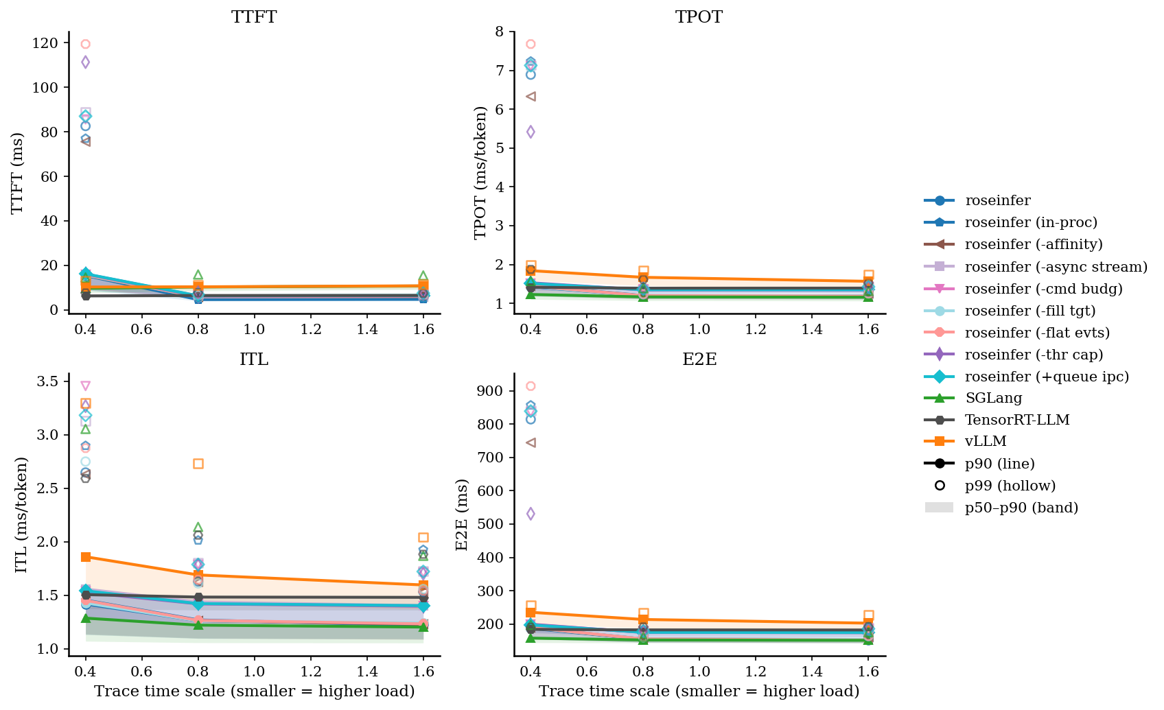
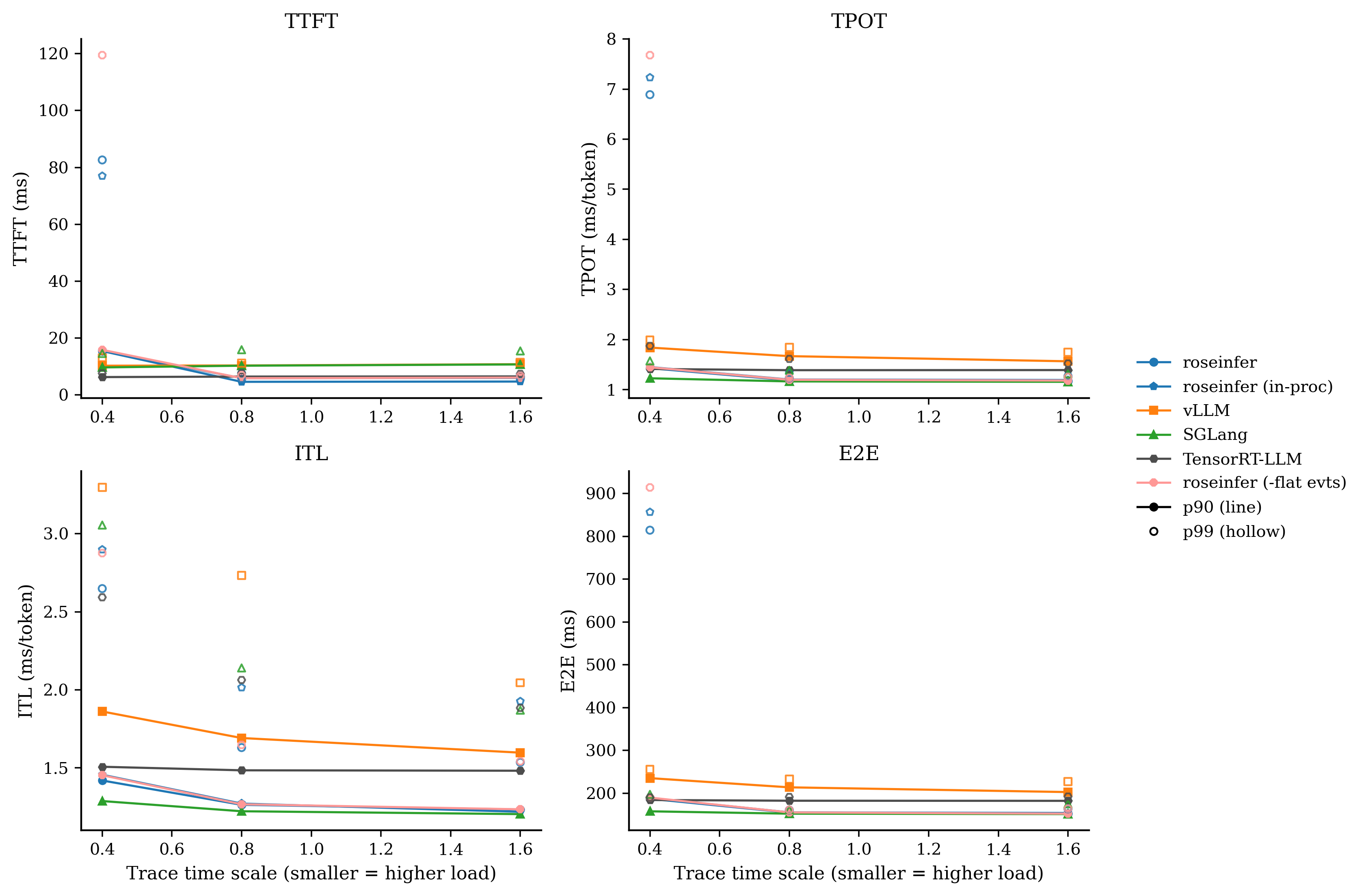
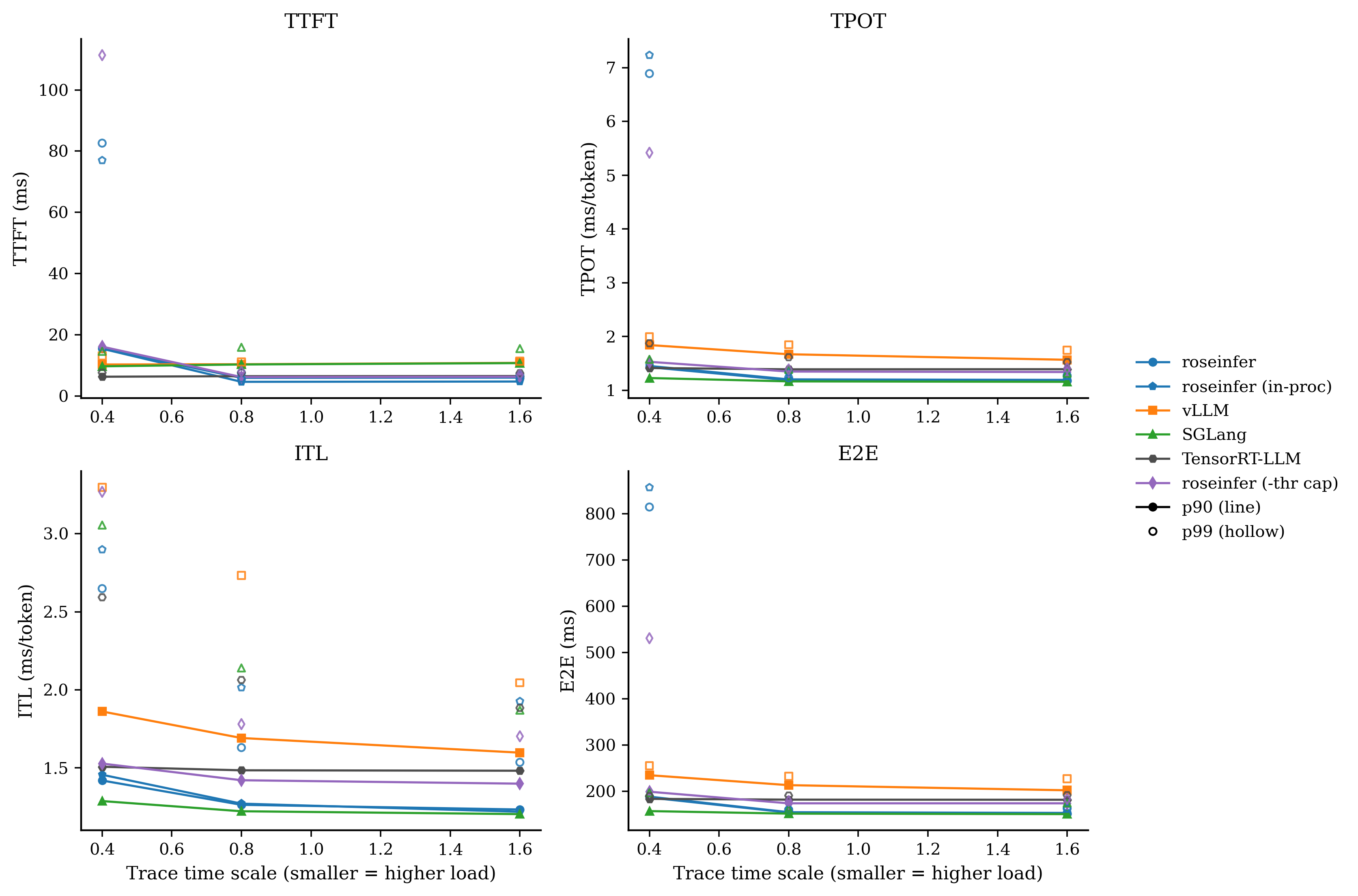
Online：延迟

p90 曲线 + p50–p90 band，空心点为 p99。

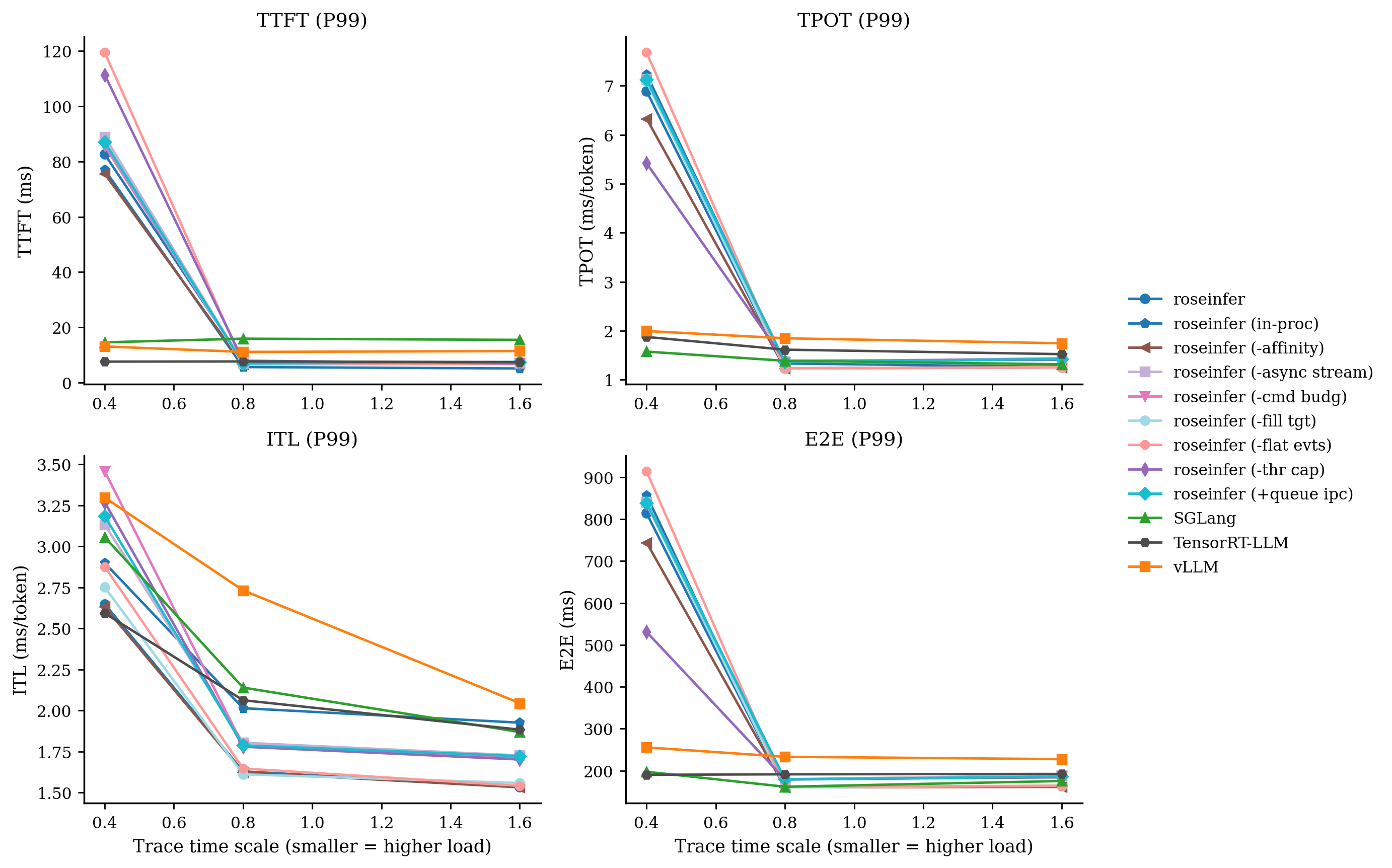
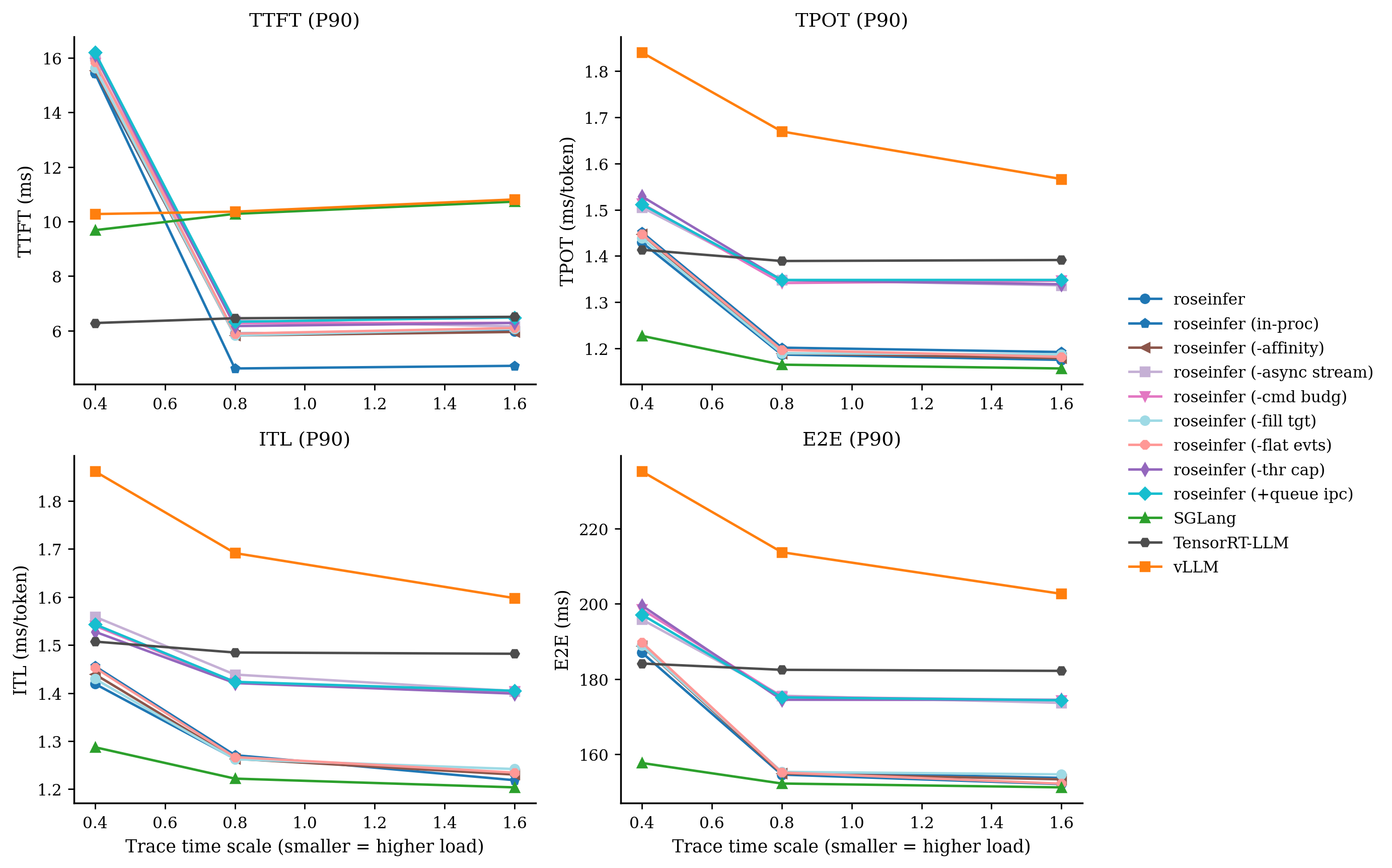
为了更直观看 tail（以及避免 band 把图挤得太花），我另外画了两张“只看一个分位”的版本：

Online：只看 P99

Online：只看 P90

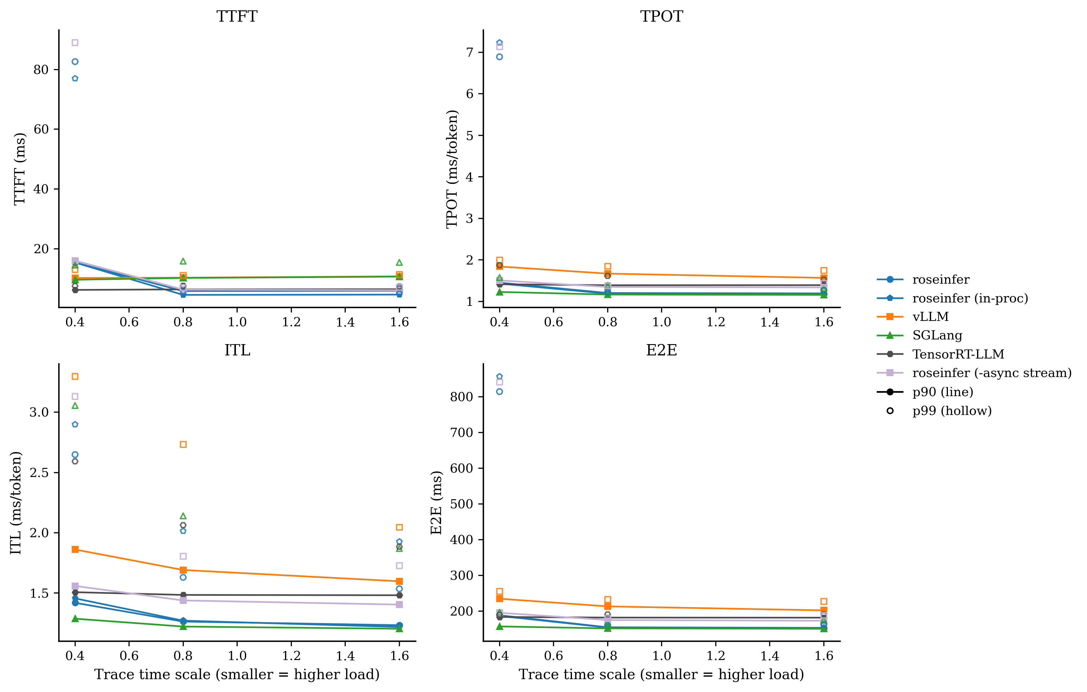
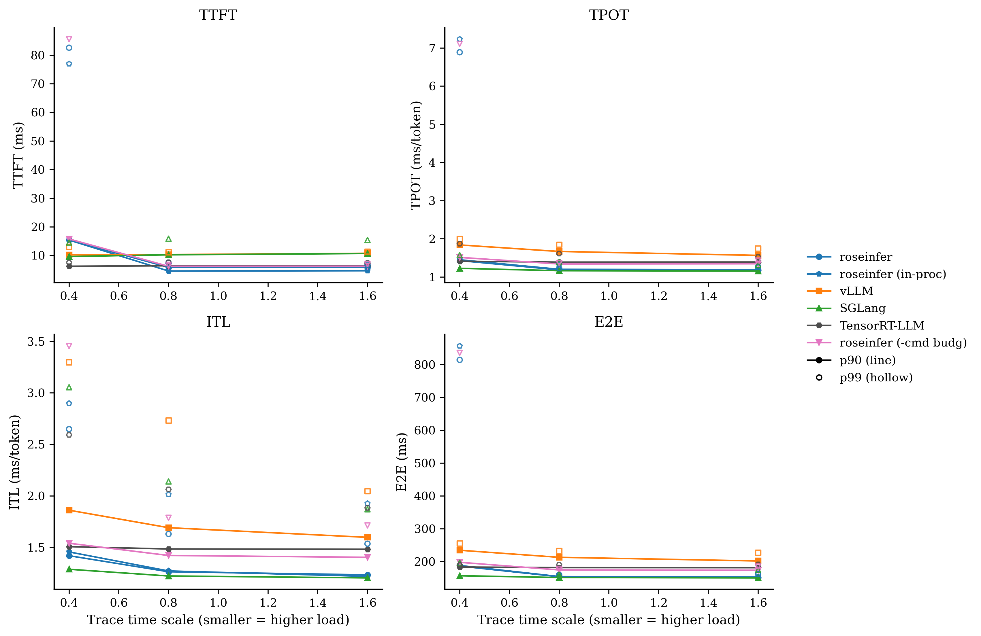
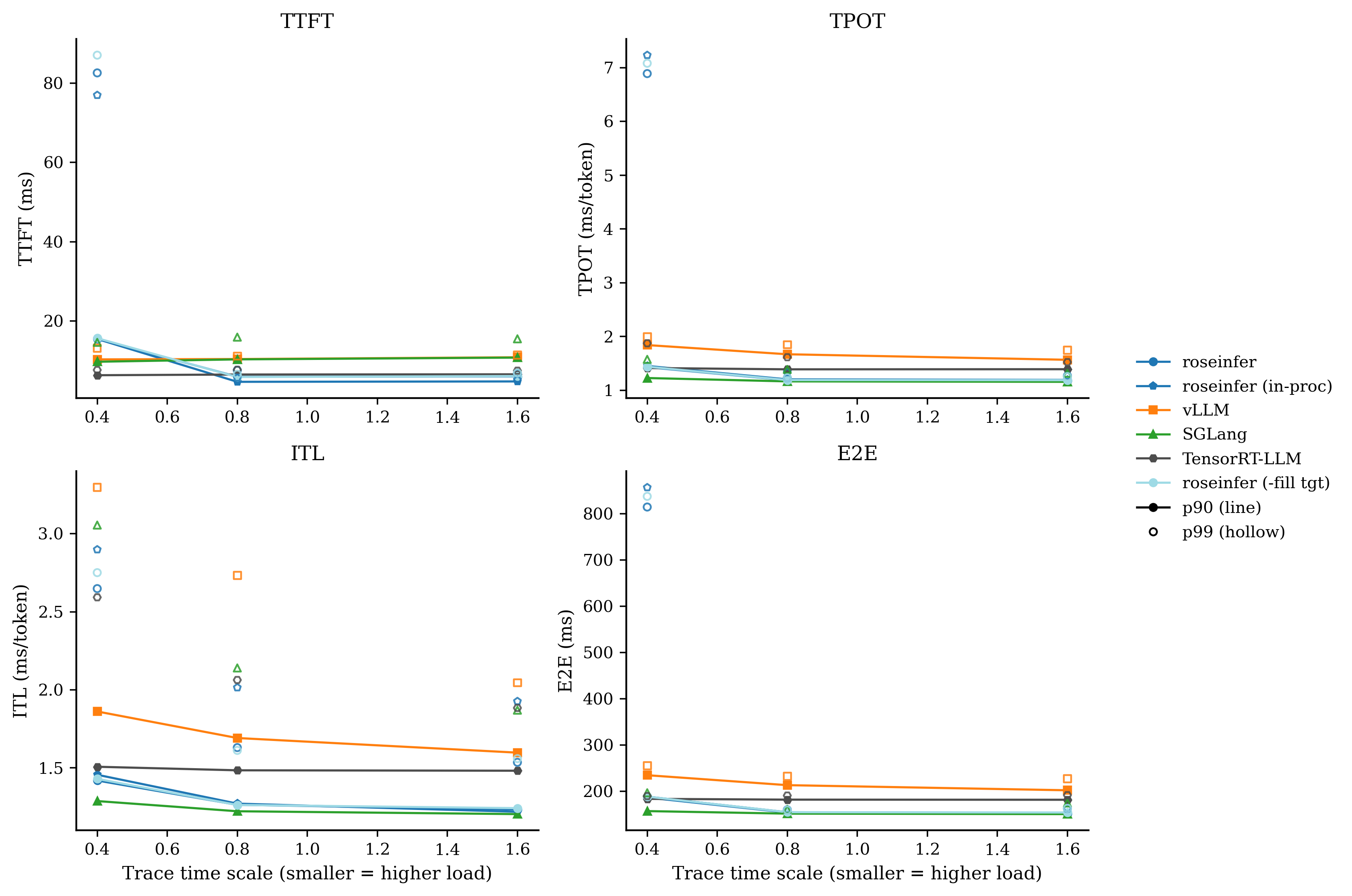
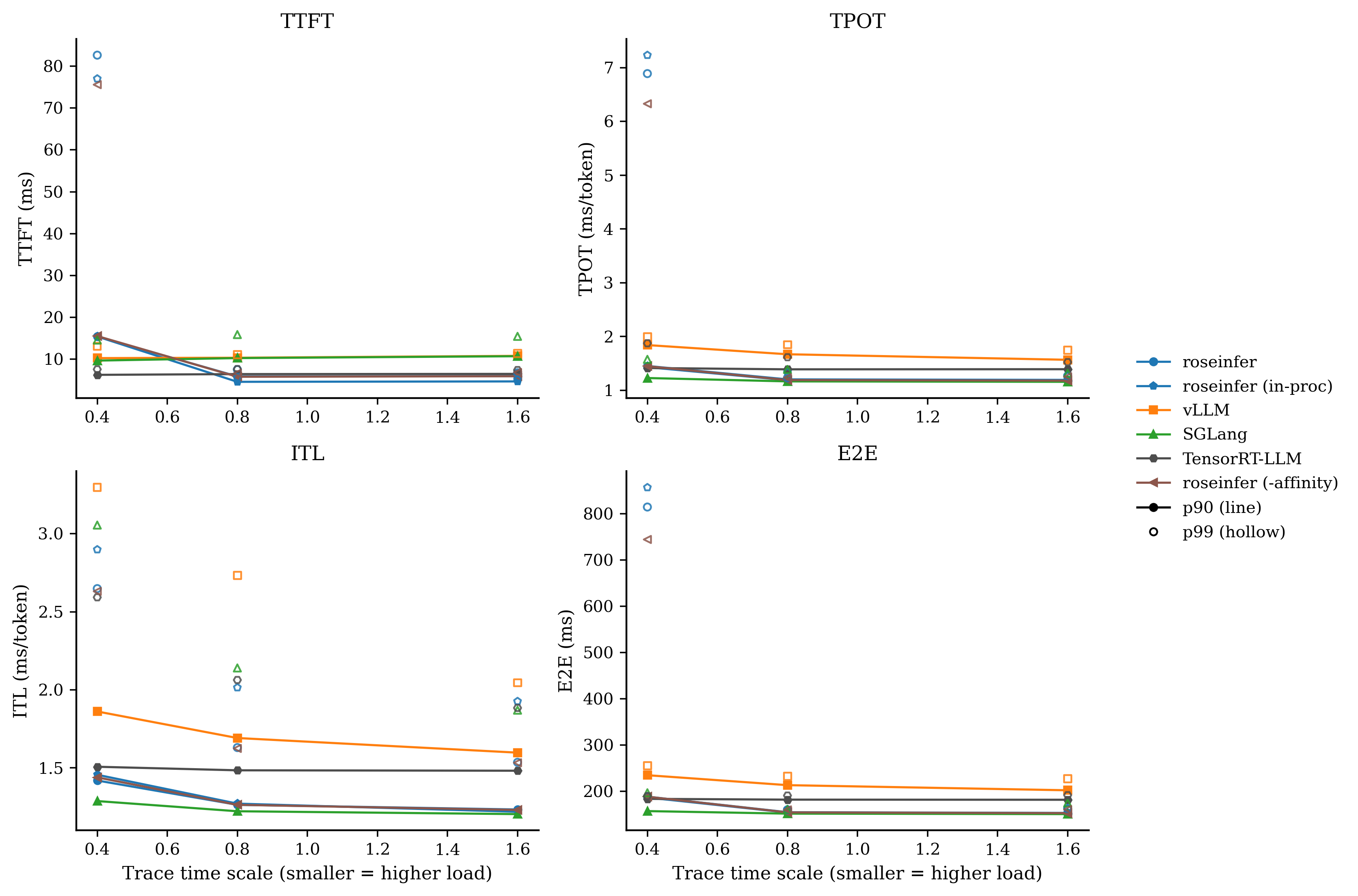
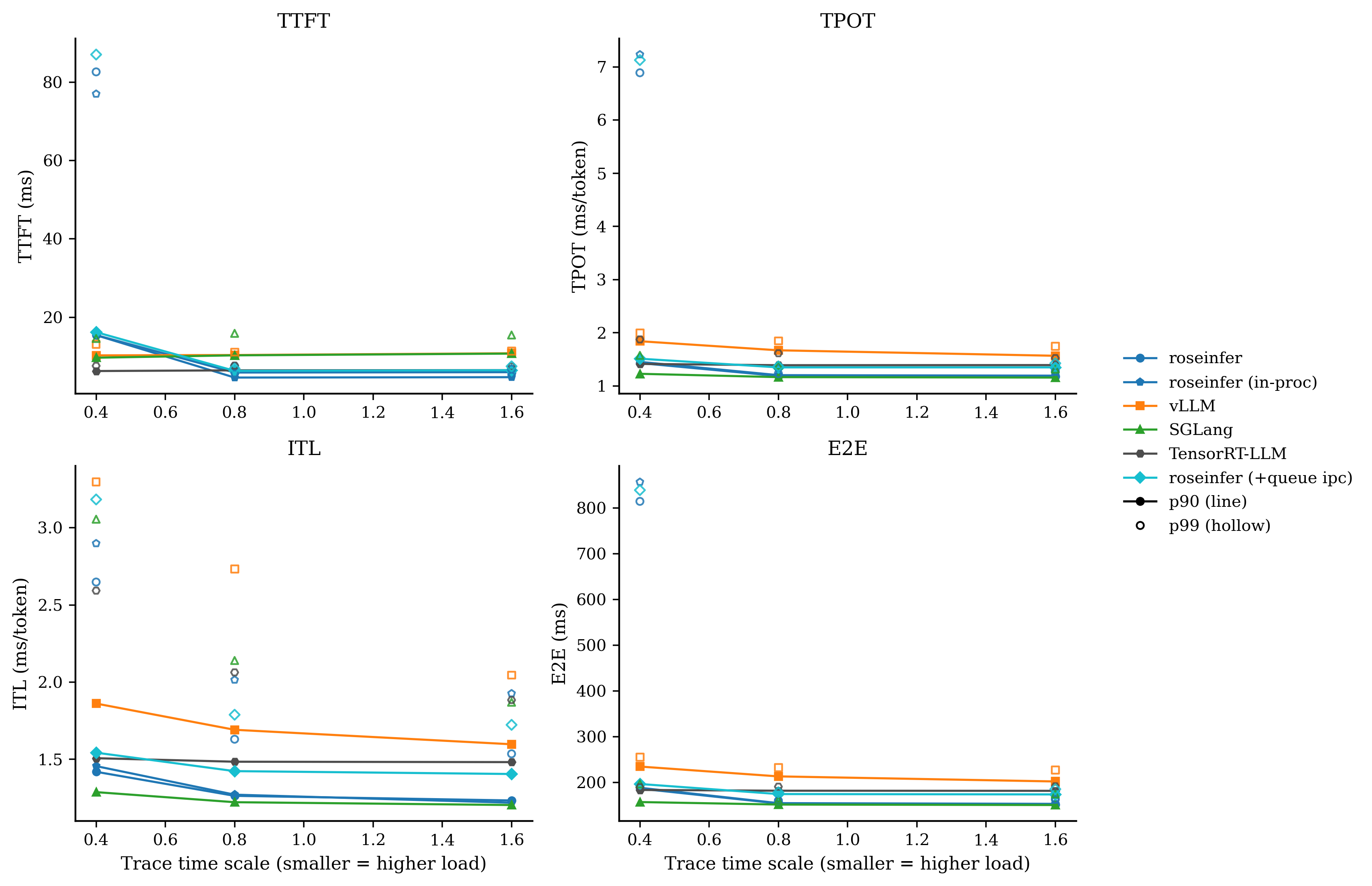
Online：单点对比图，固定 5 个 baseline + 1 个变体

每张图里固定放：roseinfer / roseinfer (in-proc) / vLLM / SGLang / TensorRT-LLM，然后额外加一个“单点变体”，让 P90/P99 的差异更容易被肉眼抓出来。

对比：-async stream

对比：-flat evts

对比：-cmd budg

对比：-fill tgt

对比：-affinity

对比：-thr cap

对比：+queue ipc

原始数据表格

scale	backend	TTFT p50/p90/p99 (ms)	TPOT p50/p90/p99 (ms)	ITL p50/p90/p99 (ms)	E2E p50/p90/p99 (ms)
0.40	roseinfer	8.89/15.44/82.62	1.19/1.43/6.89	1.13/1.42/2.65	155.08/187.03/814.29
0.40	roseinfer (in-proc)	8.85/15.43/76.99	1.20/1.45/7.23	1.14/1.46/2.90	155.74/188.87/856.59
0.40	roseinfer (-affinity)	9.27/15.54/75.57	1.19/1.45/6.33	1.14/1.44/2.63	154.91/188.75/744.20
0.40	roseinfer (-async stream)	9.74/16.07/88.98	1.35/1.51/7.13	1.28/1.56/3.13	174.47/195.80/840.56
0.40	roseinfer (-cmd budg)	9.63/15.82/85.61	1.34/1.51/7.11	1.28/1.54/3.46	173.61/198.54/835.71
0.40	roseinfer (-fill tgt)	9.20/15.62/87.10	1.19/1.44/7.08	1.13/1.43/2.75	155.83/188.85/837.33
0.40	roseinfer (-flat evts)	9.34/15.86/119.46	1.19/1.45/7.68	1.14/1.45/2.88	156.26/189.74/914.13
0.40	roseinfer (-thr cap)	9.49/16.11/111.37	1.35/1.53/5.42	1.28/1.53/3.27	174.68/199.52/530.98
0.40	roseinfer (+queue ipc)	9.98/16.20/87.04	1.35/1.51/7.13	1.28/1.54/3.18	174.20/197.10/838.82
0.40	SGLang	7.67/9.69/14.58	1.10/1.23/1.57	1.07/1.29/3.06	144.10/157.67/197.26
0.40	TensorRT-LLM	5.68/6.28/7.60	1.38/1.41/1.87	1.37/1.51/2.59	180.05/184.11/190.06
0.40	vLLM	9.21/10.28/13.09	1.59/1.84/1.99	1.53/1.86/3.30	200.58/235.18/255.43
0.80	roseinfer	5.17/5.90/7.53	1.12/1.19/1.23	1.10/1.26/1.63	145.87/154.57/160.55
0.80	roseinfer (in-proc)	4.00/4.62/5.63	1.12/1.20/1.33	1.10/1.27/2.01	145.24/155.24/160.99
0.80	roseinfer (-affinity)	5.04/5.83/6.65	1.11/1.19/1.23	1.10/1.26/1.62	145.30/154.86/160.37
0.80	roseinfer (-async stream)	5.21/6.37/7.01	1.27/1.35/1.37	1.24/1.44/1.80	161.46/175.56/179.46
0.80	roseinfer (-cmd budg)	5.28/6.28/6.78	1.27/1.34/1.36	1.25/1.42/1.79	162.93/175.27/178.53
0.80	roseinfer (-fill tgt)	5.21/5.83/6.52	1.11/1.19/1.23	1.10/1.26/1.61	145.43/155.31/160.07
0.80	roseinfer (-flat evts)	5.32/5.89/6.98	1.11/1.20/1.24	1.10/1.27/1.65	145.77/155.13/161.13
0.80	roseinfer (-thr cap)	5.16/6.17/7.93	1.27/1.35/1.39	1.24/1.42/1.78	160.76/174.47/179.42
0.80	roseinfer (+queue ipc)	5.40/6.33/6.91	1.27/1.35/1.37	1.24/1.42/1.79	162.73/175.13/178.96
0.80	SGLang	8.50/10.28/15.90	1.07/1.17/1.39	1.06/1.22/2.14	143.34/152.21/161.56
0.80	TensorRT-LLM	5.77/6.46/7.66	1.37/1.39/1.61	1.36/1.48/2.06	179.11/182.43/191.21
0.80	vLLM	9.20/10.36/11.11	1.45/1.67/1.85	1.42/1.69/2.73	187.58/213.70/233.04
1.60	roseinfer	5.36/5.99/6.76	1.11/1.18/1.27	1.09/1.23/1.54	143.86/152.06/163.43
1.60	roseinfer (in-proc)	4.18/4.71/5.12	1.12/1.19/1.26	1.10/1.22/1.93	143.92/153.71/162.79
1.60	roseinfer (-affinity)	5.39/5.95/6.86	1.11/1.18/1.25	1.09/1.23/1.53	144.18/153.32/161.17
1.60	roseinfer (-async stream)	5.48/6.16/7.10	1.25/1.34/1.44	1.23/1.40/1.73	161.54/173.63/188.90
1.60	roseinfer (-cmd budg)	5.43/6.29/7.02	1.26/1.35/1.43	1.23/1.40/1.71	161.16/174.38/185.72
1.60	roseinfer (-fill tgt)	5.49/6.07/6.83	1.11/1.19/1.25	1.09/1.24/1.56	144.35/154.65/163.69
1.60	roseinfer (-flat evts)	5.41/6.10/6.74	1.11/1.18/1.25	1.09/1.23/1.54	143.76/152.17/163.99
1.60	roseinfer (-thr cap)	5.41/6.29/6.93	1.26/1.34/1.41	1.23/1.40/1.70	161.23/174.45/183.97
1.60	roseinfer (+queue ipc)	5.80/6.48/7.48	1.26/1.35/1.42	1.23/1.40/1.72	161.60/174.33/185.84
1.60	SGLang	9.12/10.73/15.47	1.06/1.16/1.32	1.06/1.20/1.87	143.18/151.19/175.24
1.60	TensorRT-LLM	5.95/6.51/7.43	1.37/1.39/1.52	1.36/1.48/1.88	179.02/182.16/192.10
1.60	vLLM	9.55/10.81/11.40	1.37/1.57/1.74	1.37/1.60/2.05	182.75/202.63/227.41

我自己的读法很直接：

• -async stream 在 scale=0.8/1.6 上把 E2E/TPOT 拉得很明显（线程海的代价）；
• +queue ipc、-flat evts 这类改动对 p99 很诚实：热路径的 Python/IPC 开销就是会放大到尾部；
• baseline（全开）在 roseinfer variants 里终于变得像 baseline：它应该最稳、也确实最稳。

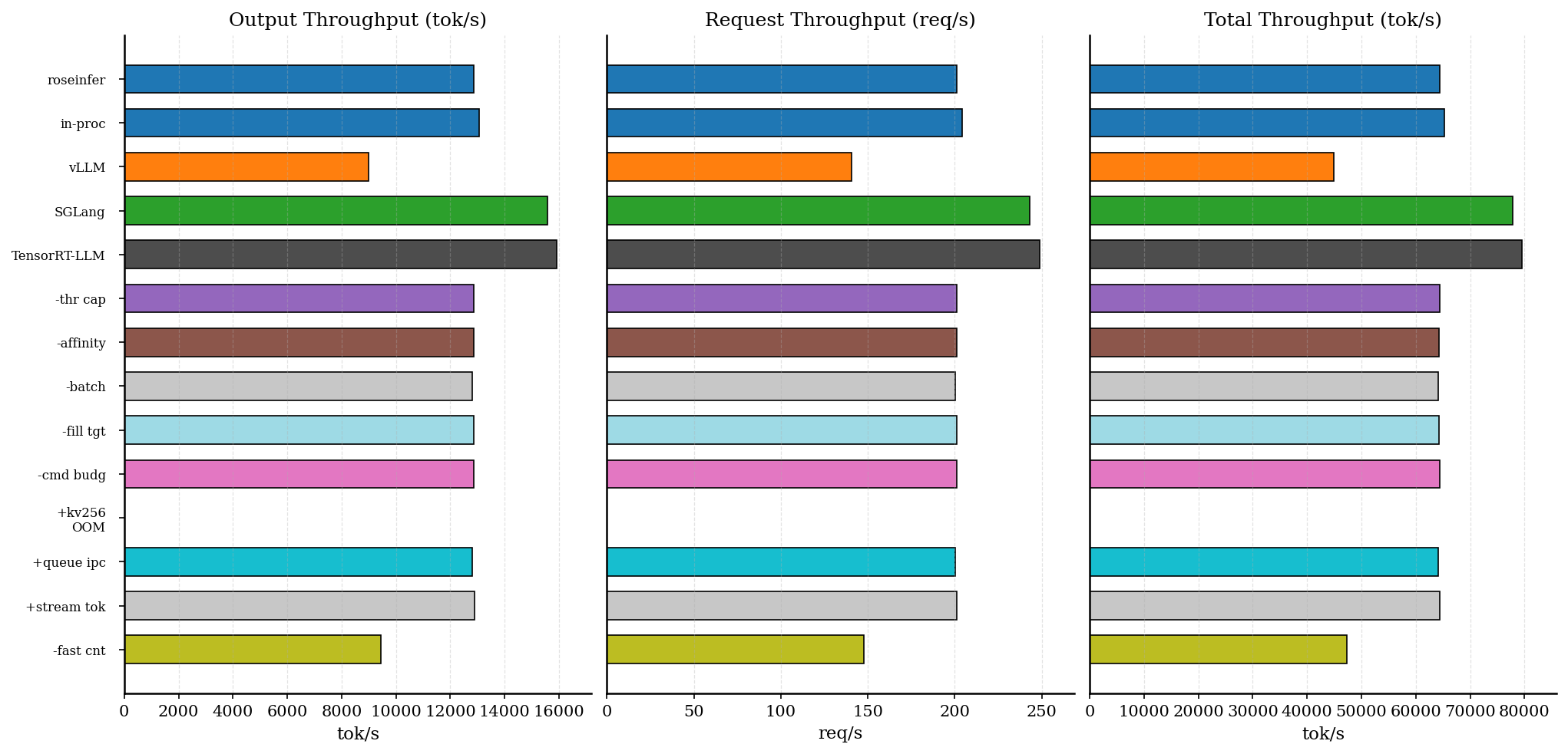
Offline：吞吐 - finish-only

原始数据表格

backend	req/s	output tok/s	total tok/s	total latency (s)
roseinfer	201.14	12872.99	64364.95	0.636
roseinfer (in-proc)	204.01	13056.84	65284.22	0.627
roseinfer (+kv256)	0.00	0.00	0.00	9.071
roseinfer (-affinity)	201.03	12866.10	64330.52	0.637
roseinfer (-batch send)	200.21	12813.58	64067.92	0.639
roseinfer (-cmd budg)	201.06	12867.85	64339.24	0.637
roseinfer (-fill tgt)	200.99	12863.17	64315.84	0.637
roseinfer (-thr cap)	201.16	12874.52	64372.58	0.636
roseinfer (+queue ipc)	200.26	12816.90	64084.48	0.639
roseinfer (-fast cnt)	147.75	9456.12	47280.59	0.866
roseinfer (+stream tok)	201.26	12880.77	64403.85	0.636
SGLang	243.20	15564.48	77822.40	0.526
TensorRT-LLM	248.69	15916.24	79581.21	0.515
vLLM	140.44	8988.14	44940.70	0.911

offline 这张我更关心两点：

1) MP baseline 已经非常接近 in-proc（差距大概就是“多进程固定税”的那点尾巴，约 1–2%）；
2) -fast cnt 一关就暴跌，说明我们之前确实在用“在线粒度”做“离线统计”，纯浪费 CPU。

（+kv256 这次直接 OOM：它属于风险项，默认就应该关，ablation 里留着只是提醒自己“别手痒”。）

---

一个很蠢但很关键的坑：为什么你会看到 vLLM 对比“前后翻转”？

这段我必须写，不然我自己也不信我跑出来的数。

我早期有一轮 offline（同一个 git_rev=5099b2b）跑出来 roseinfer < vLLM，后来又变成 roseinfer > vLLM。看起来像“优化点差不多但结论乱跳”，实际根因是：我把一次性开销算进了计时。

具体表现是：

• 旧的 offline 跑数没有 warmup_full_batch（warmup 没覆盖到真正的 shape/path）；
• CUDA Graph capture / Triton compile / allocator warmup 这些一次性成本被计进了 timed region；
• vLLM 这类系统本身 init/warmup 覆盖更完整，所以受影响更小；
• 结果就是：只有 roseinfer 看起来突然慢了 2×，排名被污染。

我现在统一用带 warmup_full_batch=True 的那轮作为最终 offline 数据（就是上面那张表），这才是 steady-state 吞吐。

---

Profiling：怎么采？文件在哪？我建议先看什么？

这部分强烈建议配合 073 一起看（profiling harness 的设计和坑在那篇写得更全）。

1) 我这次跑出来的文件位置示例

Online：

• 结果：outputs/benchmarks/serving/online_20251228_231859/online_results.json
• profile 索引：outputs/benchmarks/serving/online_20251228_231859/profile_manifest.json
• torch traces：
  • roseinfer：outputs/benchmarks/serving/online_20251228_231859/profiles/torch/roseinfer/trace.json
  • vLLM：outputs/benchmarks/serving/online_20251228_231859/profiles/torch/vllm/*.pt.trace.json.gz
  • SGLang：outputs/benchmarks/serving/online_20251228_231859/profiles/torch/sglang/*.trace.json.gz
• nsys：outputs/benchmarks/serving/online_20251228_231859/profiles/nsys/<backend>/nsys.nsys-rep

Offline：

• 结果：outputs/benchmarks/serving/offline_20251229_001108/offline_results.json
• profile 索引：outputs/benchmarks/serving/offline_20251229_001108/profile_manifest.json
• torch：outputs/benchmarks/serving/offline_20251229_001108/profiles/torch/<backend>/*trace.json*
• nsys：outputs/benchmarks/serving/offline_20251229_001108/profiles/nsys/<backend>/nsys.nsys-rep

2) SGLang offline 的“三段式 profile”怎么处理？

SGLang 的 Engine 是 TokenizerManager(main) + Scheduler(proc) + Detokenizer(proc) 三段式。

我一开始犯过一个很蠢的错：在 wrapper 进程里 with torch.profiler.profile 包住 engine.generate()，采到的基本是“主进程空转”；真正的 GPU work 在 scheduler 子进程里，trace 里看不到。

现在 offline harness 的做法是：直接调用 engine.tokenizer_manager.start_profile(...)，让 scheduler 自己把 trace 导出来（文件名里会带 TP-0）。如果你想看全进程树的系统行为，nsys 更靠谱。

3) 我看 profile 的顺序

1) 先看 GPU timeline 有没有大 gap：有 gap 基本就是 CPU 把 GPU 饿住了；
2) 再看 NVTX/record_function range（roseinfer 已经在 engine/mp loop 里打了很多 tag）：

• roseinfer.mp.drain_cmds / roseinfer.mp.add_requests / roseinfer.mp.step
• roseinfer.model.forward* / roseinfer.scheduler.*
  3) 如果你在追 tail：重点看 CPU runnable/blocked + IPC send/recv 有没有 backpressure。

---

复现命令

Online：

python benchmarks/serving/online_compare.py --model gpt2 --device cuda --dtype fp16 --gpu 0 --n 200 --scales 0.4,0.8,1.6 --backends roseinfer,vllm,sglang,trtllm --roseinfer-compare-engine-process --roseinfer-compare-mp-ablations --profile both --profile-n 16 --profile-output-len 32

Offline：

python benchmarks/serving/offline_compare.py --model gpt2 --device cuda --dtype fp16 --gpu 0 --trtllm-backend tensorrt --num-prompts 128 --input-len 256 --output-len 64 --temperature 0.7 --top-p 0.9 --top-k 50 --seed 42 --tensor-parallel-size 1 --max-batch-size 256 --warmup-prompts 8 --ignore-eos --backends roseinfer_mp,roseinfer,vllm,sglang,trtllm --roseinfer-compare-mp-ablations --profile both --profile-num-prompts 8 --profile-input-len 256 --profile-output-len 32

---

小结与下一步

这篇收尾我想留三个结论：

1) 多进程的难点不是“拆”，是“拆完以后把工程税压到看不见”：线程池、绑核、IPC、loop 公平性，哪个没调对都会把你所有 micro-opt 一票否决。
2) baseline（全开）现在终于像 baseline：在 roseinfer variants 里最稳，ablation 的语义也统一成了 -xxx/+yyy。
3) MP baseline 仍然比 in-proc 略慢一点点（主要是固定税），但已经到了我愿意继续往上迭代的位置。

下一步我自己最想继续抠的方向也很明确：

• 进一步压 IPC 固定税（甚至考虑更激进的 shared memory / ring buffer）；
• 把 tokenizer/detok 的 CPU 热点再细分拆一遍（对标 SGLang 那种三段式的优缺点）；
• 用 profile 把 “CPU launch gap” 和 “engine loop 的 Python 分配” 再做一次跨框架对比，看看还有哪些肉眼可见的 gap。