Mixture of Experts
稀疏 Mixture of Experts 将模型总容量与每个 token 的激活计算部分解耦。真正的设计对象不是“有多少专家”,而是路由、容量、通信、负载和学习信号组成的整体系统。
从 early expert mixtures、Sparsely-Gated MoE 到 Switch 与 DeepSeekMoE 的变化见条件计算与稀疏专家;关键路由与 capacity 语义的可执行缩影见稀疏 MoE 深读。
路由
设 token 表示为 \(x\),router logits 为
经过 top-\(k\) 选择得到集合 \(\mathcal T(x)\),MoE 输出可写为
top-\(k\) 是离散选择;未被选中的专家通常不接收主任务梯度。router 的初始化、噪声、精度和 tie-breaking 都会影响早期专家分化。
细粒度与共享专家
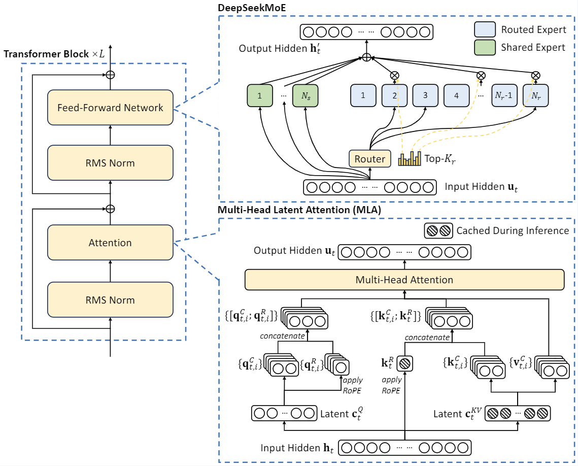
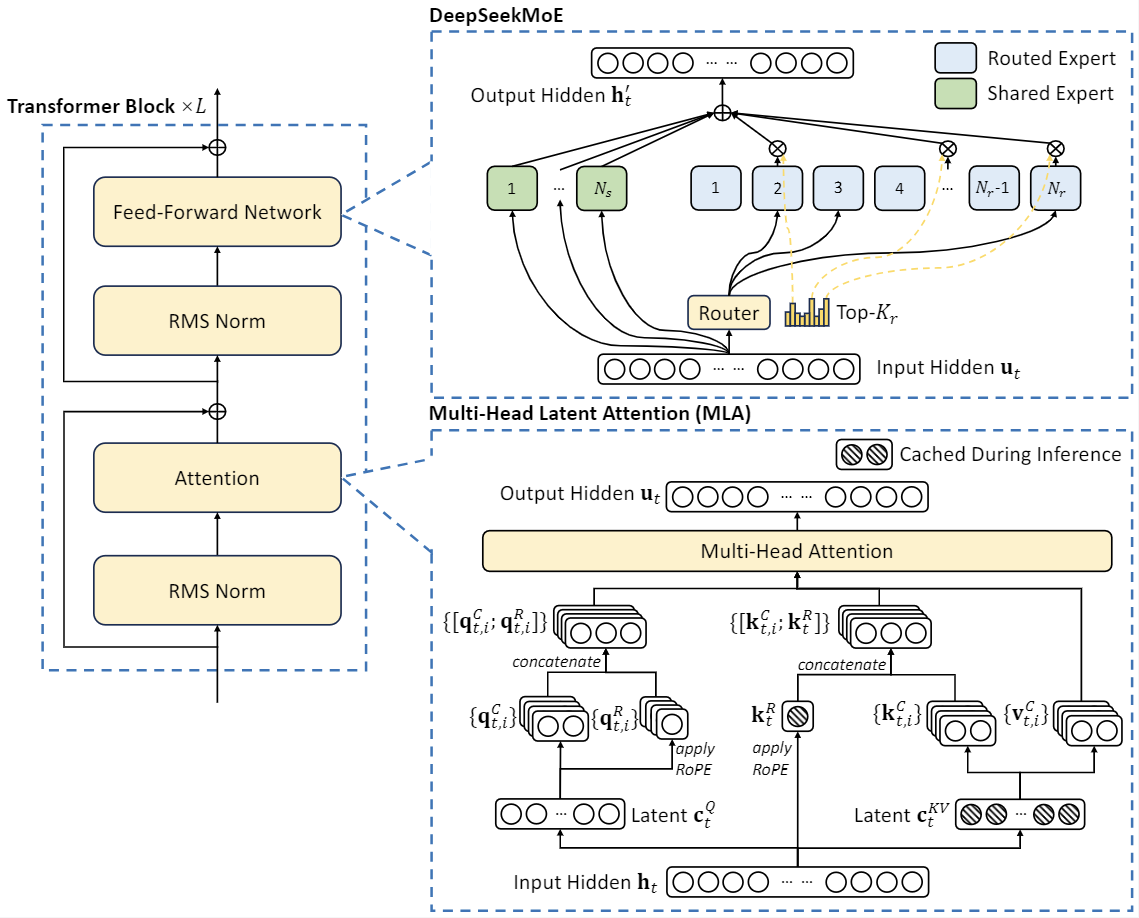
将一个大 FFN 拆成更多小专家,可以用更丰富的组合表达相近激活参数量;代价是路由元数据、kernel 粒度和通信消息更碎。共享专家对所有 token 激活,承担通用变换;路由专家则学习条件化分工。DeepSeekMoE 是细粒度与共享专家组合的代表。
LatentMoE:把路由压进窄通道
普通 MoE 让每个被选专家接收完整 hidden width \(d\);当 expert pool 和 top-\(k\) 同时扩大时,dispatch bytes 与专家权重流量随之增长。LatentMoE 把通用变换留在 full-width shared experts,把条件化路由放进宽度 \(\ell<d\) 的 latent path:
于是 routed expert 的输入、输出和跨 rank token payload 都可按 \(\ell\) 设计,而 shared path 仍在 \(d\) 维承载公共知识。低维路由不是免费容量:若 \(\ell\) 太小,所有 specialist 共享同一个投影瓶颈; 若 active expert 数增大,dispatch 次数、元数据和小 GEMM 利用率仍会恶化。
Kimi K3 技术报告中的 Stable LatentMoE 取 \(d=7168\)、\(\ell=3584\),在 896 个 routed experts 中每 token 激活 16 个,并 始终激活 2 个 full-width shared experts。它在 routed aggregate 与 up-projection 之间加入 RMSNorm,使 \(W_\uparrow\) 看到的尺度较少依赖本次选中了哪些专家及其 gate weight;再与 SiTU-GLU 和后文的 Quantile Balancing 共同处理极稀疏训练中的 activation 与负载问题。LatentMoE 到 Stable LatentMoE 深读 区分了原作与 K3 增量,并从 balanced assignment dual 推导 QB;完整模型实例见 Kimi K3。
Latent routed path reference
下面用单层线性 expert 缩写 routed/shared FFN,只保留 down-project、top-\(k\) dispatch、 RMSNorm 和 up-project 的 shape 语义。真实 expert 应替换为完整 gated FFN。
import torch
import torch.nn.functional as F

def latent_moe(x, down, up, router, routed, shared, top_k):
    tokens, width = x.shape
    experts, latent, _ = routed.shape
    assert down.shape == (latent, width) and up.shape == (width, latent)
    assert router.shape == (experts, width) and shared.shape[1:] == (width, width)
    z = F.linear(x, down)
    score, index = F.linear(x, router).sigmoid().topk(top_k, dim=-1)
    gate = score / score.sum(-1, keepdim=True)
    aggregate = torch.zeros_like(z)
    for slot in range(top_k):
        weight = routed[index[:, slot]]
        expert_output = torch.einsum("noi,ni->no", weight, z)
        aggregate += gate[:, slot, None] * expert_output
    normalized = aggregate * aggregate.square().mean(-1, keepdim=True).add(1e-6).rsqrt()
    shared_output = sum(F.linear(x, weight) for weight in shared)
    return shared_output + F.linear(normalized, up), normalized

torch.manual_seed(0)
x = torch.randn(6, 8)
args = (torch.randn(4, 8), torch.randn(8, 4), torch.randn(5, 8))
routed, shared = torch.randn(5, 4, 4), torch.randn(2, 8, 8)
output, normalized = latent_moe(x, *args, routed, shared, top_k=2)
assert output.shape == x.shape and torch.isfinite(output).all()
torch.testing.assert_close(normalized.square().mean(-1), torch.ones(6), atol=2e-5, rtol=0)
这里没有 capacity、expert parallel、GLU、bias 或 padding;它只锁定 full-width 与 latent-width 的 边界。RMSNorm 稳定的是 aggregate 的输入尺度,不会修复路由塌缩、专家内部 outlier 或通信拥塞。
容量与溢出
若 batch 中共有 \(N\) 个 token、\(E\) 个专家、每 token 选择 \(k\) 个专家,平均负载为
训练实现常为每个专家设置 capacity
其中 \(c\) 是 capacity factor。负载超过容量时,可以丢 token、路由到备选专家、增加 padding 或使用无固定容量的动态 kernel。每种策略都改变质量、内存和最坏时延。
最小语义实现
sparse_moe 接收扁平 token x:[N,D]、router weight [E,D] 和 expert weights [E,D,D],返回加权输出、实际专家负载、top-\(k\) 索引与被保留的 assignment。capacity 的优先级先看 routing rank:全体 token 的 top-1 先于任何 top-2;同一 rank 内再按 token 输入顺序保留。
import torch
import torch.nn.functional as F
def sparse_moe(x, router, experts, top_k=2, capacity=None):
    if x.ndim != 2 or router.ndim != 2 or experts.ndim != 3: raise ValueError("invalid ranks")
    tokens, hidden = x.shape
    expert_count = experts.shape[0]
    if router.shape != (expert_count, hidden): raise ValueError("router/expert mismatch")
    if experts.shape[1:] != (hidden, hidden): raise ValueError("expert shape mismatch")
    if not isinstance(top_k, int) or not 1 <= top_k <= expert_count:
        raise ValueError("invalid top_k")
    if capacity is not None and (not isinstance(capacity, int) or capacity <= 0):
        raise ValueError("capacity must be a positive integer")
    score, index = F.linear(x, router).float().topk(top_k, dim=-1)
    gate = score.softmax(-1).to(x.dtype)
    output, load = torch.zeros_like(x), torch.zeros(expert_count, dtype=torch.long)
    kept = torch.zeros_like(index, dtype=torch.bool)
    for slot in range(top_k):
        for expert_id, expert in enumerate(experts):
            token = torch.where(index[:, slot] == expert_id)[0]
            if capacity is not None:
                token = token[:max(capacity - load[expert_id].item(), 0)]
            if token.numel():
                output[token] += gate[token, slot, None] * F.linear(x[token], expert)
                load[expert_id] += token.numel()
                kept[token, slot] = True
    return output, load, index, kept
x = torch.tensor([[3., 0.], [2., 0.], [0., 3.]])
router, experts = torch.eye(2), torch.eye(2).repeat(2, 1, 1)
_, load, _, kept = sparse_moe(x, router, experts, top_k=2, capacity=1)
assert kept.tolist() == [[True, False], [False, False], [True, False]]
assert load.tolist() == [1, 1]
try: sparse_moe(x, torch.randn(3, 2), experts, top_k=2)
except ValueError: pass
else: raise AssertionError("router/expert mismatch must fail")
kept 的断言锁定了 top-1 优先于 top-2、同 slot 按 token 顺序的容量语义。丢弃后不重归一化残余 gate;备选路由、其他 token-dropping 优先级和稳定 tie-breaking 都会改变结果。生产实现还要用 permutation 与 all-to-all 取代 Python 循环,并核对反向、跨 rank 容量和负载统计;具体张量变换见分布式与容错:MoE dispatch 与 combine。
负载均衡
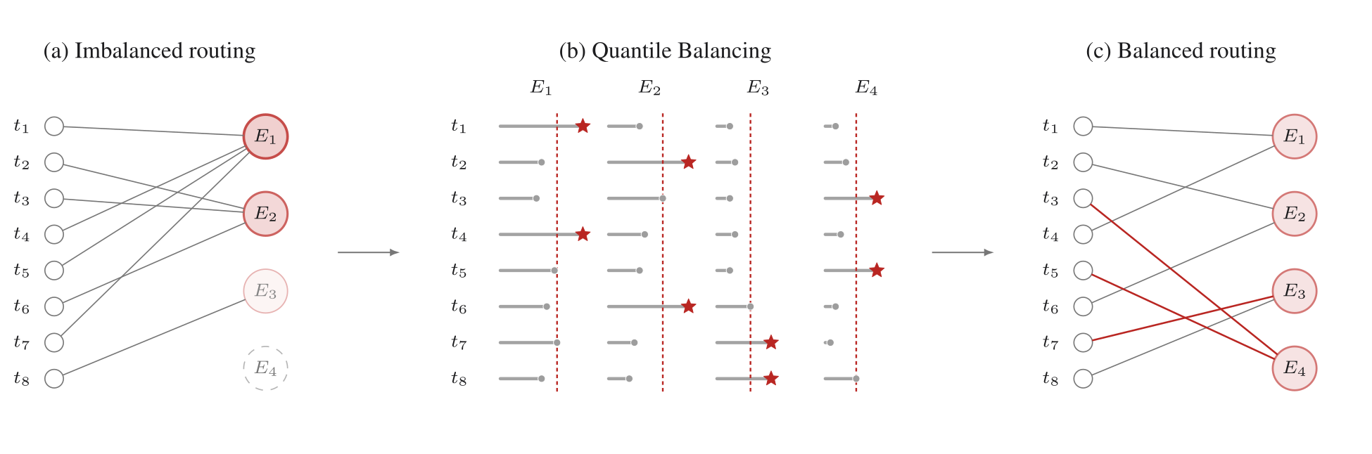
只优化语言建模损失时,router 可能把大量 token 送到少数专家。经典辅助项同时考察路由概率和实际分配,鼓励专家接收接近均匀的负载;但辅助梯度也可能干扰主目标。
Auxiliary-Loss-Free Load Balancing 在 top-\(k\) 前为每个专家增加动态 bias,根据近期负载更新 bias,而不让均衡信号直接反传到主 router score。它减少一种干扰来源,却没有消除容量、局部拥塞和跨节点流量问题。
Quantile Balancing:从追赶负载到直接估计阈值
固定步长的 loss-free update 只根据“过载还是欠载”移动 bias,步长小会追赶缓慢,步长大又会振荡。 Quantile Balancing(QB)把 bias 解释为每个专家的录取阈值,并从当前 score distribution 直接估计 下一步阈值。对 \(m\) 个 token、\(n\) 个专家、每 token 选 \(k\) 个,目标负载为
router 先给 raw score \(s_i=\operatorname{Sigmoid}(W_rx_i)\)。selection 使用 bias,mixture weight 却只使用 raw score:
因此 \(b\) 只移动离散 dispatch 边界,不直接改专家输出权重或 router 的主任务梯度。当前 bias \(b^{(t)}\) 下,对每个 token 取 biased Top-\((k+1)\) 的第 \(k+1\) 个值作为 cutoff \(\alpha_i^{(t)}\);expert \(j\) 若满足 \(s_{i,j}+\tilde b_j>\alpha_i^{(t)}\) 就进入候选集合。令恰好 \(q\) 个 margin 超过阈值,可得
去均值不改变 top-\(k\);新 bias 只在 下一次 训练 step 生效,不能用当前 batch 推导后再回头路由同一 batch。推理冻结最终 bias,也不再计算 quantile。
下面采用“第 \(q+1\) 大 margin”的离散定义,避免把不同库的 quantile interpolation 约定藏起来。 无 tie 的小例子中,一次更新把负载从 \((2,1,3,2)\) 调到目标 \((2,2,2,2)\)。
import torch

def quantile_balancing_bias(scores, bias, top_k):
    tokens, experts = scores.shape
    assert 0 < top_k < experts and tokens * top_k % experts == 0
    cutoff = (scores + bias).topk(top_k + 1, dim=-1).values[:, -1]
    target = tokens * top_k // experts
    margin = scores - cutoff[:, None]
    candidate = -margin.sort(dim=0, descending=True).values[target]
    return candidate - candidate.mean()

def expert_load(scores, bias, top_k):
    index = (scores + bias).topk(top_k, dim=-1).indices.flatten()
    return torch.bincount(index, minlength=scores.size(1))

torch.manual_seed(13)
scores = torch.sigmoid(torch.randn(8, 4))
bias = torch.zeros(4)
assert expert_load(scores, bias, 1).tolist() == [2, 1, 3, 2]
next_bias = quantile_balancing_bias(scores, bias, 1)
assert expert_load(scores, next_bias, 1).tolist() == [2, 2, 2, 2]
torch.testing.assert_close(next_bias.mean(), torch.tensor(0.))
全局 step 可能包含数百万 token,直接 gather 全部 margin 不现实。K3 用每专家直方图近似分位数: 各 rank/gradient-accumulation micro-batch 只累加 bin count,step 末对 \(nB\) 个整数做一次 all-reduce,再从全局累计计数恢复 quantile。取 \(B=1000\) 时,估计误差不超过一个 bin width,通信量 与 token 数无关。直方图解决的是全局阈值估计成本;capacity、节点内局部热点与不同 expert 的实际 kernel 时间仍需单独监控。
均衡至少有三种口径:
- 全局 token 数是否均匀;
- 每个 expert-parallel group 内是否均匀;
- 实际 wall-clock 是否均匀。
token 数相同的专家也可能因序列形状、kernel 或节点拥塞产生不同耗时。
Expert Parallel
典型前向包含:
local tokens
-> router and permutation
-> all-to-all dispatch
-> local expert GEMM
-> all-to-all combine
-> inverse permutation
通信量与 token 表示宽度、top-\(k\)、dtype 和跨节点比例相关。专家太小会使 GEMM 无法饱和,专家太大又限制分片与负载弹性。实际系统常将 tensor parallel、data parallel 与 expert parallel 组合,并尝试把 dispatch/combine 与其他计算重叠。
训练稳定性
- router logits 使用过低精度可能放大 top-\(k\) 边界抖动;
- 高学习率会让专家分工快速漂移;
- 某些 token 类别可能长期绑定少数专家,形成过拟合;
- batch 太小或数据源分布剧变,会让负载统计噪声很大;
- shared expert 与 routed expert 的尺度不一致,会改变残差分布;
- checkpoint 恢复后若路由随机性或数据游标改变,专家负载可能突然跳变。
应监控每专家 token 数、路由概率、drop rate、容量利用率、专家输出范数、跨节点流量和最慢专家时延,而不只看总 loss。
DeepSeek-V4 的路由改动
DeepSeek-V4 延续 DeepSeekMoE 的细粒度 routed experts 与 shared expert,但在 V3 配方上改了四处:
- affinity 从 \(\operatorname{Sigmoid}(z)\)改成 \(\sqrt{\operatorname{Softplus}(z)}\);
- 保留 auxiliary-loss-free bias balancing,同时加入很小的 sequence-wise balance loss,防止单条长序列内部极端失衡;
- 取消 routing target node 数约束,把节点放置交给重新设计的并行系统;
- 最前三个 MoE layer 按 input token ID 做固定 hash routing,以确定性路由替代早期 dense FFN。
Flash 与 Pro 都使用 1 个 shared expert、256 / 384 个 routed experts、top-6;expert hidden 分别为 2048 / 3072。Hash 层仍是 MoE 计算,只是 expert ID 不由可学习 router 决定;它降低早期路由不稳定,不代表这些层会自动得到语义专家分工。
报告没有给出这些改动各自的规模消融,也没有公开 sequence loss 的完整归约细节。系统侧的 wave dispatch、pull-based activation 与通信阈值见 MegaMoE。
推理
MoE decode 的激活 FLOPs 可以较低,但全部专家权重仍需驻留、分片或按需加载。小 batch 下每个专家收到的 token 很少,GEMM 利用率下降;大 batch 又增加 KV 和尾延迟。量化、专家缓存与 speculative routing 都要在真实路由分布上评测。
比较表
报告 MoE 至少包含:
total and activated parameters
number and size of routed/shared experts
top-k and router normalization
capacity and overflow policy
load-balancing objective or bias
expert-parallel topology
communication dtype and overlap
training token distribution
quality, throughput, tail latency and memory
Switch Transformer 展示了 top-1 稀疏路由,DeepSeek-V3 则把细粒度专家、无辅助损失均衡和系统配方结合。替代序列架构见稀疏与替代架构,分布式实现见模型并行。
Reference
- DeepSeekMoE
- LatentMoE: Toward Optimal Accuracy per FLOP and Parameter
- Auxiliary-Loss-Free Load Balancing Strategy for Mixture-of-Experts
- Switch Transformers
- DeepSeek-V3
- Kimi K3 Technical Report
- Hash Layers for Large Sparse Models
- DeepSeek-V4: Towards Highly Efficient Million-Token Context Intelligence