从 LatentMoE 到 Stable LatentMoE：窄路由、稳定激活与分位数均衡

稀疏 MoE 常用“每个 token 只激活少量参数”描述效率，但真实服务还要搬运 expert 权重，并在 expert-parallel ranks 间传输 routed token。专家池和 top-\(k\) 继续增大时，FLOPs 可能仍可控，显存带宽与 all-to-all payload 却会先成为瓶颈。

LatentMoE 从这个系统约束出发，把 full model width 与 routed expert width 解耦；Kimi K3 技术报告随后把该结构扩展为 Stable LatentMoE，重点处理超大专家池下的内部激活和路由负载稳定性。两者是一条清晰的演进链，却不是同一项工作：

层面	原始 LatentMoE	K3 Stable LatentMoE 的增量
routed path	down-project → latent experts → up-project	routed aggregate 后、up-project 前加入 RMSNorm
shared path	full-width shared experts	保留 full-width，并在 K3 中固定为 2 个
expert activation	论文按实验配置使用既有 FFN activation	引入 SiTU-GLU，平滑限制两个乘法分支
router/load balance	原作实验使用既有 balancing recipe	Sigmoid raw score、selection-only bias 与 Quantile Balancing
目标	accuracy per FLOP / parameter / serving cost	在 896/16 的极端稀疏设置中稳定训练和负载

因此不能把 RMSNorm、SiTU-GLU 或 QB 反向归到 LatentMoE 原论文，也不能把 K3 的具体宽度和 expert 数当成原作的固定定义。

原始 LatentMoE：只压缩 Routed Path

令 token 表示为 \(x\in\mathbb R^d\)，latent width 为 \(\ell<d\)。原始 LatentMoE 让 router 仍从 full-width \(x\) 计算 expert score，但实际被 dispatch 的 payload 先经过共享 down-projection：

\[ z=W_\downarrow x\in\mathbb R^\ell. \]

若 \(\mathcal T_k(x)\) 是选中的 routed expert，原作的核心结构可写成

\[ y_{\mathrm{routed}} = W_\uparrow \left( \sum_{i\in\mathcal T_k(x)} p_iE_i^{\mathrm{routed}}(z) \right), \]

\[ y =y_{\mathrm{routed}} +\sum_{j=1}^{N_s}E_j^{\mathrm{shared}}(x). \]

routed expert 的输入、输出与跨 rank payload 都在 \(\ell\) 维；shared experts、router 和其他非 routed 计算仍在 \(d\) 维。这样做有两个直接后果：

• expert 权重读取与 routed payload 不再被 full hidden width \(d\) 锁死；
• 省下的参数、FLOPs 或通信预算可以用于更多 experts 或更大的 top-\(k\)。

但 \(\ell\) 不是越小越好。所有 specialist 共享 \(W_\downarrow/W_\uparrow\) 形成的信息瓶颈；当 \(\ell\) 低于任务相关的有效特征秩，扩大专家池也无法恢复被投影删除的信息。原论文因此把 latent width、expert 数和 top-\(k\) 作为联合设计变量，而不是孤立地做低秩压缩。NVIDIA LatentMoE 研究页进一步从低并发权重带宽和高吞吐 all-to-all 两种工作负载解释了这项选择。

完整 MoE 参数与 dispatch 语义见稀疏 MoE，expert parallel 的 permutation、通信与 GEMM 边界见 MoE 系统。

K3 的 Stable 增量

K3 把 routed expert 扩大到 896 个、每 token 激活 16 个，latent width 为 3584，full hidden width 为 7168，并始终激活 2 个 full-width shared expert。报告指出，这种 routed path 串联 down-projection、gated multi-branch expert 和 up-projection，形成多次连续矩阵乘；在其规模下，vanilla 路径出现内部 activation explosion，而近千 expert 也放大了负载均衡的迟滞。

Stable LatentMoE 用三项增量分别处理这两个问题：

1. routed aggregate 后加入 RMSNorm；
2. expert FFN 使用 SiTU-GLU；
3. router bias 使用 Quantile Balancing。

它们分别作用于 aggregate scale、expert 内部坐标和离散 dispatch，不能互相替代。

RMSNorm 放在 Aggregate 与 Up-projection 之间

K3 的 routed branch 为

\[ u = \sum_{i\in\mathcal T_k(x)} p_iE_i^{\mathrm{routed}}(W_\downarrow x), \]

\[ y = \sum_{j=1}^{N_s}E_j^{\mathrm{shared}}(x) +W_\uparrow\operatorname{RMSNorm}(u). \]

原作直接把 \(u\) 输入 \(W_\uparrow\)；K3 新增的 RMSNorm 让 up-projection 看到更稳定的 RMS scale。它不会让不同 expert mixture 的方向相同，也不会修复 router collapse；它只减少“选中了哪些 expert、raw mixture weight 多大”造成的整体尺度漂移。

SiTU-GLU 平滑限制乘法坐标

SwiGLU 的 gate 线性因子和 up branch 都无界。K3 对两者分别应用 smooth cap：

\[ \operatorname{softcap}(a;\beta)=\beta\tanh(a/\beta), \]

\[ \operatorname{SiTU\text{-}GLU}(a,b) = \left[ \beta_1\tanh(a/\beta_1)\odot\sigma(a) \right] \odot \left[ \beta_2\tanh(b/\beta_2) \right]. \]

报告取 \(\beta_1=4,\beta_2=25\)，因而逐坐标满足

\[ \left\|\operatorname{SiTU\text{-}GLU}(a,b)\right\|_\infty \le \beta_1\beta_2=100. \]

软上界改变的是远离原点后的数值几何。左侧公式显示两个乘法分支分别经过 tanh softcap；右侧曲线则把局部近似与远端饱和放在同一坐标系中。红线在原点附近仍贴近 SwiGLU，却不会像无界分支一样持续增长。图源：Kimi K3 Technical Report, Figure 4, p. 7；© 2026 Moonshot AI，Kimi K3 License。

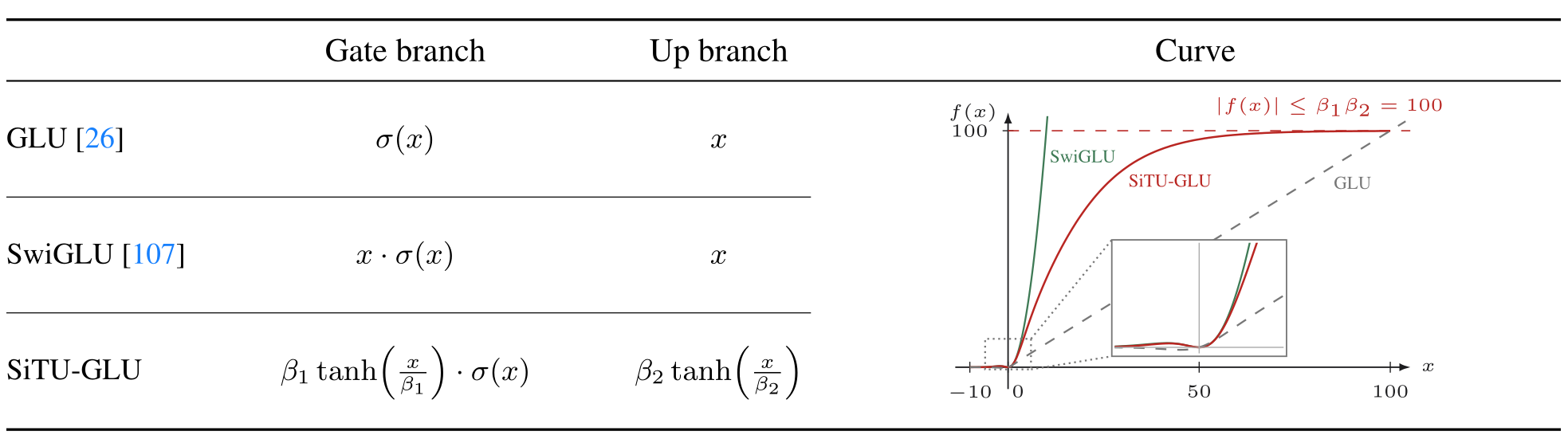
在原点附近 \(\beta\tanh(x/\beta)=x+O(x^3)\)，所以它保留 SwiGLU 的局部一阶行为；进入大幅值区间后，tanh 平滑饱和。与 hard clamp 相比，它没有离散边界，但饱和区梯度仍会减小，不能把“输出有界”理解成“任意深度和低精度都不会溢出”。

最小结构 Reference

下面用小型线性 expert 固定四个语义：shared path 保持 full width，routed path 在 latent width 中 dispatch，selection bias 不进入 mixture weight，RMSNorm 位于 aggregate 与 up-projection 之间。

import torch
import torch.nn.functional as F

def raw_score_route(raw_score, bias, top_k):
    index = (raw_score + bias).topk(top_k, dim=-1).indices
    chosen = raw_score.gather(-1, index)
    return index, chosen / chosen.sum(-1, keepdim=True)

def stable_latent_moe(x, down, up, router, experts, shared, bias, top_k):
    tokens, width = x.shape
    count, latent, expert_in = experts.shape
    if expert_in != latent or down.shape != (latent, width):
        raise ValueError("routed experts must stay in the latent width")
    if up.shape != (width, latent) or router.shape != (count, width):
        raise ValueError("projection and router shapes do not align")
    z = F.linear(x, down)
    raw = F.linear(x, router).sigmoid()
    index, mixture = raw_score_route(raw, bias, top_k)
    aggregate = torch.zeros_like(z)
    for slot in range(top_k):
        weight = experts[index[:, slot]]
        value = torch.einsum("toi,ti->to", weight, z)
        aggregate += mixture[:, slot, None] * value
    rms = aggregate.square().mean(-1, keepdim=True).add(1e-6).rsqrt()
    routed = F.linear(aggregate * rms, up)
    shared_value = sum(F.linear(x, weight) for weight in shared)
    return shared_value + routed, aggregate * rms

raw = torch.tensor([[.9, .8, .1]])
index, mixture = raw_score_route(raw, torch.tensor([-1., 0., 2.]), 2)
assert index.tolist() == [[2, 1]]
torch.testing.assert_close(mixture, torch.tensor([[1 / 9, 8 / 9]]))
torch.manual_seed(7)
x = torch.randn(5, 6)
y, normalized = stable_latent_moe(
    x, torch.randn(3, 6), torch.randn(6, 3), torch.randn(4, 6),
    torch.randn(4, 3, 3), torch.randn(2, 6, 6), torch.zeros(4), 2
)
assert y.shape == x.shape
torch.testing.assert_close(normalized.square().mean(-1), torch.ones(5), atol=2e-5, rtol=0)

这个 reference 没有实现真实 gated expert；SiTU-GLU 的完整线性分支、capacity、all-to-all 和 backward 属于下一层实现。它也不复现 K3 的参数规模，只锁定结构位置和 score/bias 语义。

Router：Selection 与 Mixture 分家

K3 对 token \(x_i\) 计算无 bias 的 Sigmoid score

\[ s_i=\operatorname{Sigmoid}(W_rx_i). \]

expert bias \(b\) 只参与 top-\(k\) selection：

\[ \mathcal T_i =\operatorname{arg\,topk}(s_i+b). \]

选中 expert 的 combine weight 仍来自 raw score：

\[ p_{i,j} = \frac{s_{i,j}} {\sum_{r\in\mathcal T_i}s_{i,r}}, \qquad j\in\mathcal T_i. \]

因此 bias 可以移动离散 dispatch 边界，却不直接混入 expert 输出权重。主任务梯度仍通过被选中的 raw score 路径传播；bias update 是训练状态，不由语言建模 loss 优化。这里的“分家”不是说 bias 没有模型影响——更换 selected expert 本身就会改变输出——而是避免把负载控制量连续叠加到 mixture amplitude。

从 Balanced Assignment 到 Convex Dual

设一个 batch 有 \(m\) 个 token、\(n\) 个 routed expert，每个 token 选择 \(k\) 个 expert。令 \(x_{i,j}\in\{0,1\}\) 表示 token \(i\) 是否分配给 expert \(j\)。若

\[ q=\frac{mk}{n} \]

为整数，最大 raw-score 的严格均衡 assignment 是

\[ \max_x \sum_{i=1}^{m}\sum_{j=1}^{n}x_{i,j}s_{i,j}, \]

subject to

\[ \sum_jx_{i,j}=k, \qquad \sum_ix_{i,j}=q. \]

把 \(x_{i,j}\) 放松到 \([0,1]\) 后得到 bipartite \(b\)-matching linear program；其多面体具有整数最优点，所以 relaxation 不损失这个 assignment 的整数语义。为 token constraint 引入自由变量 \(\alpha_i\)，为 expert constraint 引入 \(\beta_j\)，可得 convex dual：

\[ \mathcal L(\alpha,\beta) = \sum_{i,j} \max(0,s_{i,j}-\alpha_i-\beta_j) +k\sum_i\alpha_i +q\sum_j\beta_j. \]

给定 \(\beta\)，每个 \(\alpha_i\) 的子问题是分段线性的；当恰有 \(k\) 个 \(s_{i,j}-\beta_j\) 位于阈值之上时达到 coordinate minimum。因此可取该行第 \(k+1\) 大值：

\[ \alpha_i^\star =\operatorname{quantile}_{1-k/n}(s_i-\beta). \]

给定 \(\alpha\)，对 expert \(j\) 同理：

\[ \beta_j^\star =\operatorname{quantile}_{1-k/n}(s_{:,j}-\alpha). \]

在无 tie 时，\(x_{i,j}=1\) 当且仅当 \(s_{i,j}-\alpha_i-\beta_j>0\)。最终 deployment 只需保存 expert threshold \(\beta\)，或等价 bias \(b=-\beta\)；token threshold \(\alpha\) 只是当前 batch 的中间变量。

这解释了 QB 与固定步长 loss-free update 的关系：后者只使用 expert load error 的符号做一步 SignSGD，QB 则跳到同一个 dual coordinate 的精确 minimizer。精确的是单个 coordinate update，不是说一次交替更新必然求出任意有限 batch 的全局 assignment。

Quantile Balancing 的一步更新

K3 不单独运行完整 assignment solver。当前 step 使用 bias \(b^{(t)}\) 做 Top-\((k+1)\)：

\[ \alpha_i^{(t)} = \operatorname{k{+}1\text{-}largest} \left(s_i+b^{(t)}\right). \]

前 \(k\) 项照常 dispatch，第 \(k+1\) 项是 token cutoff。对 expert \(j\) 定义 margin

\[ m_{i,j}=s_{i,j}-\alpha_i^{(t)}. \]

要让恰好 \(q\) 个 margin 在新 bias 后超过 cutoff，候选更新为

\[ \widehat b_j^{(t+1)} = -\operatorname{quantile}_{1-k/n}(m_{:,j}), \]

再利用 common shift 不改变 top-\(k\) 的性质去均值：

\[ b^{(t+1)} = \widehat b^{(t+1)} -\operatorname{mean}\!\left(\widehat b^{(t+1)}\right)\mathbf1. \]

新 bias 只在下一训练 step 生效。用当前 batch 算完 bias 后重新路由同一 batch，会让 action 与生成它的 policy state 不一致，也会把算法从 causal controller 改成 batch-level assignment。

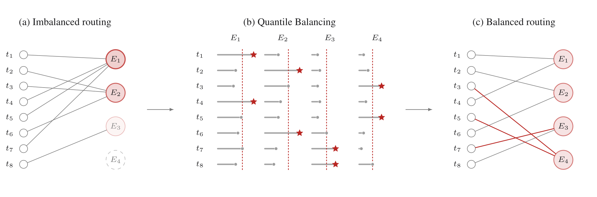
从左到右读一次 coordinate update。当前选择先形成 (4, 3, 1, 0) 的 expert load；中间按 expert 列寻找 margin threshold；红星与红边标出 selection boundary 真正改变的部分，结果成为 (2, 2, 2, 2)。这是单个 batch 的说明性例子，不是一次更新必然全局收敛的证明。图源：Kimi K3 Technical Report, Figure 5, p. 8；© 2026 Moonshot AI，Kimi K3 License。

Exact Coordinate Reference

下面明确采用“第 \(q+1\) 大 margin”作为离散 quantile，并拒绝非整数 target 与阈值 tie。实际系统若允许 tie，必须固定 secondary key 或 fractional assignment 规则，不能依赖未指定的 topk 顺序。

import torch

def qb_coordinate_bias(raw_score, old_bias, top_k):
    tokens, experts = raw_score.shape
    routes = tokens * top_k
    if not 0 < top_k < experts or routes % experts:
        raise ValueError("QB requires an integral equal-load target")
    target = routes // experts
    cutoff = (raw_score + old_bias).sort(dim=-1, descending=True).values[:, top_k]
    margin = raw_score - cutoff[:, None]
    ordered = margin.sort(dim=0, descending=True).values
    if torch.isclose(ordered[target - 1], ordered[target]).any():
        raise ValueError("boundary ties need an explicit assignment rule")
    candidate = -ordered[target]
    return candidate - candidate.mean()

def routed_load(raw_score, bias, top_k):
    index = (raw_score + bias).topk(top_k, dim=-1).indices.flatten()
    return torch.bincount(index, minlength=raw_score.size(1))

torch.manual_seed(21)
score = torch.sigmoid(torch.randn(8, 4))
old = torch.zeros(4)
assert routed_load(score, old, 1).tolist() == [3, 0, 2, 3]
new = qb_coordinate_bias(score, old, 1)
assert routed_load(score, new, 1).tolist() == [2, 2, 2, 2]
torch.testing.assert_close(new.mean(), torch.tensor(0.))
try:
    qb_coordinate_bias(torch.ones(4, 2), torch.zeros(2), 1)
except ValueError:
    pass
else:
    raise AssertionError("ties must not silently choose an arbitrary expert")

这个小例子恰好在一次更新后完全均衡；它不是对所有新 batch 的保证。若 score distribution 在相邻 step 漂移，bias 仍可能落后，只是 coordinate update 通常比固定步长更直接。

Histogram All-reduce

全局 batch 的 \(m\times n\) margin 可能跨 data-parallel ranks 和 gradient-accumulation micro-batches，直接 gather 既占内存又让通信随 token 数增长。K3 实际维护的是 required bias

\[ r_{i,j}=\alpha_i-s_{i,j}=-m_{i,j}. \]

由于 \(s_{i,j}\in(0,1)\)，而 cutoff 来自某个 \(s_{i,j'}+b_{j'}\)，若当前 bias 范围为 \([b_{\min},b_{\max}]\)，则

\[ r_{i,j}\in[b_{\min}-1,\ b_{\max}+1]. \]

K3 每 step 用这个自适应范围建立每 expert 的均匀 histogram。每个 rank 在本地、跨 micro-batch 累加整数 count，step 末只对 \(nB\) 个 bin count 做一次 all-reduce；所有 rank 再从同一 pooled cumulative count 找到目标 bin，并在 bin 内插值。报告使用 \(B=1000\)，未插值时 quantile 误差由一个 bin width 上界控制。

这里有一个常见错误：

\[ \operatorname{quantile}\left(\bigcup_rD_r\right) \ne \frac1R\sum_r\operatorname{quantile}(D_r). \]

应该 all-reduce 可加的 histogram count，而不是平均各 rank 的 quantile。前者对 token 怎样切到 ranks/micro-batches 不敏感；后者会被 shard size 与局部分布扭曲。整数 count 的 dtype 还必须覆盖完整 global step，bin range 更新和 bias update 也要在所有 rank 上使用同一个 step boundary。

四个不能略过的边界

Tie

LP 可以有多个同分最优 assignment；普通 topk 的 tie-breaking 可能随 kernel、dtype 或 rank 改变。严格“每 expert 恰好 \(q\)”依赖无 tie 假设。低精度量化 score、直方图边界或大量相同 token 都会提高 tie 概率，应使用稳定 secondary key、明确的 fractional/capacity rule，或接受并报告残余 imbalance。

Integer target

若 \(mk/n\) 不是整数，每个 expert 接收完全相同的整数 token 数在数学上不可能。可让 expert capacity 在 \(\lfloor mk/n\rfloor\) 与 \(\lceil mk/n\rceil\) 间分配且总和为 \(mk\)，或调整 global batch/top-\(k\)；不能用浮点 quantile 掩盖不可满足的约束。

推理冻结

训练结束后只保存最终 expert bias，inference 仍是固定 Top-\(k\)，不需要 token quantile 或 histogram collective。这保持了 deployment 接口简单，也意味着线上不能悄悄按当前请求 batch 自适应 bias；那会改变路由 policy、缓存身份与模型复现性。

分布漂移

冻结 bias 是对训练后期 score distribution 的阈值估计。语言、任务、长度、模态、量化格式或 serving batch 改变后，expert load 可能重新偏斜。应分别监控 raw score、selected load、capacity overflow 和 rank wall-clock；需要调整时走版本化再校准或继续训练，而不是在生产请求上无审计地更新 bias。

系统闭环

QB 只让 global expert token count 更接近目标，不能保证每个 rank 的执行时间相等。MoonEP 进一步在不改变 global expert identity 的前提下，用动态冗余 expert 固定 rank-level token load；两者分别作用于模型路由和执行 placement。latent payload、Quantile Balancing、MoonEP 与 grouped GEMM 的端到端关系见 MoE 系统。

同样，RMSNorm 与 SiTU-GLU 只约束 routed branch 内部数值，不能代替全模型 residual、optimizer、精度和 checkpoint 验证。SiTU-GLU 的 decoder 层位置与可执行实现见 Decoder Block，K3 中三者如何与其他架构、训练和部署机制配合见 Kimi K3。

证据边界

原始 LatentMoE 论文公开了设计空间、模型消融和部分实测/模拟 serving 分析；其参数和速度结论绑定论文模型、硬件与 simulator。K3 报告公开 Stable LatentMoE 的公式、SiTU 超参数、QB 推导与 histogram 方法，并报告 RMSNorm、SiTU-GLU、QB 的模型内使用；它没有公开足够信息来重建所有 kernel、每层完整 activation 分布、tie 处理实现或所有独立消融。

因此可以确认：

• full-width shared path 与 latent routed path 的结构分工；
• K3 在 routed aggregate 后新增 RMSNorm；
• SiTU-GLU 的数学定义和输出上界；
• QB 与 balanced assignment dual 的关系；
• exact coordinate update、global histogram 与 inference freeze。

但不能据此声称任意模型都应使用相同 \(\ell/d\)、\(\beta_1/\beta_2\)、bin 数或 EMA，也不能把 K3 的稳定训练归因于其中任一组件的孤立作用。

Reference

• LatentMoE: Toward Optimal Accuracy per FLOP and Parameter in Mixture of Experts
• NVIDIA Research LatentMoE Overview
• Kimi K3 Technical Report
• Auxiliary-Loss-Free Load Balancing Strategy for Mixture-of-Experts