Diffusion 与 Score:同一条概率路径的两种语言
Diffusion 的直觉常被压缩成“加噪,再去噪”。这句话没有错,却漏掉了最重要的统一关系:
去噪器、噪声预测器与 score estimator 都在估计同一时刻数据分布的局部几何;不同 parameterization 只是用不同坐标表达它。
这条路线并非突然出现。Score Matching 先研究不需要归一化常数的密度梯度,Denoising Score Matching 把它化为加噪样本上的回归;扩散概率模型则构造一串逐渐变成简单先验的分布,并学习反向过程。把这些放在同一组符号中,DDPM、DDIM、score SDE 与许多 sampler 的差异会清楚得多。
Score 是密度的局部指北针
分布 \(p(x)\) 的 score 定义为
它指向 log-density 增长最快的方向,但不需要知道 \(p(x)\) 的归一化常数。原始 score matching 通过分部积分把未知数据 score 从目标中消去;denoising score matching 则先用已知核扰动数据:
再回归条件核的 score:
对 Gaussian 扰动
有
这已经包含了现代 diffusion 训练的核心:随机选择噪声尺度,从带噪样本预测一个已知目标。
离散扩散:把数据逐步推向 Gaussian
Diffusion Probabilistic Models 建立了逐步破坏与反向生成框架,DDPM 给出后来最常用的 Gaussian parameterization。前向 Markov 链为
定义
便可越过中间步骤,直接采样任意时刻:
即
这条闭式边缘分布是训练可并行的原因。每个样本只需随机选 \(t\),不必真的执行 \(t\) 次加噪。
当 \(\bar\alpha_T\) 足够接近 \(0\),\(x_T\) 近似标准 Gaussian。反向条件 \(q(x_{t-1}\mid x_t,x_0)\) 也是 Gaussian;模型不知道 \(x_0\),所以用神经网络预测其均值、噪声或等价变量。
为什么简单的噪声 MSE 能工作
反向模型写成
对变分下界展开后,各时刻主要对应 Gaussian KL。DDPM 采用固定方差并重新加权,可得到常见的简化目标:
它不是随意的 denoising regression。对 variance-preserving 路径,噪声预测与 marginal score 满足
因此网络在每个噪声层级都给出“朝更高数据密度移动”的局部方向。不同 timestep 的 signal-to-noise ratio 差别很大,uniform sampling 并不意味着各尺度对梯度贡献相等;loss weighting、schedule 与 parameterization 必须作为整体设计。
\(\epsilon\)、\(x_0\) 与 \(v\) 只是坐标不同
记
预测噪声
在高噪声端 \(a_t\) 很小,从 \(\epsilon\) 恢复 \(x_0\) 会放大误差。
预测干净样本
在低噪声端 \(\sigma_t\) 很小,反向转换同样病态。
预测 velocity
常见定义为
由于
逆变换为
这里使用了 \(a_t^2+\sigma_t^2=1\)。Sampler 若把 \(v\) 当成 \(\epsilon\),shape 完全一致却会生成错误结果;checkpoint 必须显式记录 prediction_type。
从离散链到连续 SDE
Score-Based Generative Modeling through SDEs 把噪声层级写成连续时间过程:
若知道边缘分布 \(p_t(x)\) 的 score,反向时间 SDE 为
其中积分方向从 \(T\) 到 \(0\)。同一边缘分布还对应 deterministic probability-flow ODE:
这解释了“随机 diffusion sampler”和“确定性 ODE sampler”为何能共享一个 score network:它们选择不同轨迹,却可以拥有相同的时间边缘分布。实现时最危险的是时间方向。公式常以 \(dt<0\) 表示反向,代码也可用从大到小的时间网格和正差值;两种写法不能混用。
DDIM:训练边缘不变,采样耦合可以改变
DDIM 构造与 DDPM 共享 \(q(x_t\mid x_0)\) 的非 Markov 过程。给定 \(\hat x_0\) 与 \(\hat\epsilon\),一步可写为
\(\sigma_t=0\) 时轨迹确定,可跳过大量训练 timestep。少步采样的误差并非只由“步数少”决定,还取决于时间网格、prediction type、模型在高曲率区间的误差和 guidance。
DPM-Solver 进一步利用 diffusion ODE 的半线性结构构造高阶 solver;EDM 系统化讨论数据预处理、噪声 parameterization、训练权重与 sampler。两者都提醒我们:模型与采样器不是可随意拼装的独立插件。
Classifier guidance 与 classifier-free guidance
ADM 使用外部 classifier 梯度修改 conditional score:
Classifier-Free Guidance 在同一个网络中训练条件与空条件分支:
\(w=0\) 是无条件预测,\(w=1\) 是普通条件预测,\(w>1\) 外推条件方向。更高的 \(w\) 往往增强 prompt adherence,却也会降低多样性、放大饱和与解剖伪影。训练侧的 condition dropout、空 prompt 表示、负面条件与推理侧 batch 拼接顺序必须一致。
可执行的 parameterization 契约
下面只实现 forward marginal、三种 prediction 的互换和 CFG。alpha_bar 必须是按 batch 取出的累计乘积,而不是单步 \(\alpha_t\);它会被扩展到 [batch, 1, ...]。
import torch
def _batch_coeff(value, sample):
    if value.ndim != 1 or value.size(0) != sample.size(0):
        raise ValueError("coefficient must be [batch]")
    return value.reshape(value.size(0), *([1] * (sample.ndim - 1)))
def q_sample(x0, noise, alpha_bar):
    if x0.shape != noise.shape:
        raise ValueError("x0 and noise must align")
    ab = _batch_coeff(alpha_bar, x0)
    return ab.sqrt() * x0 + (1 - ab).sqrt() * noise
def targets_from_velocity(xt, velocity, alpha_bar):
    if xt.shape != velocity.shape:
        raise ValueError("xt and velocity must align")
    ab = _batch_coeff(alpha_bar, xt)
    a, sigma = ab.sqrt(), (1 - ab).sqrt()
    x0 = a * xt - sigma * velocity
    noise = sigma * xt + a * velocity
    return x0, noise
def classifier_free_guidance(unconditional, conditional, scale):
    if unconditional.shape != conditional.shape:
        raise ValueError("CFG branches must align")
    return unconditional + scale * (conditional - unconditional)
x0 = torch.tensor([[[[1., -1.]]], [[[.5, 2.]]]])
noise = torch.tensor([[[[3., 1.]]], [[[-1., .5]]]])
alpha_bar = torch.tensor([.8, .2])
xt = q_sample(x0, noise, alpha_bar)
a = _batch_coeff(alpha_bar, x0).sqrt()
sigma = _batch_coeff(1 - alpha_bar, x0).sqrt()
velocity = a * noise - sigma * x0
x0_hat, noise_hat = targets_from_velocity(xt, velocity, alpha_bar)
torch.testing.assert_close(x0_hat, x0)
torch.testing.assert_close(noise_hat, noise)
u, c = torch.zeros_like(x0), torch.ones_like(x0)
torch.testing.assert_close(classifier_free_guidance(u, c, 0), u)
torch.testing.assert_close(classifier_free_guidance(u, c, 1), c)
这不是完整 sampler。完整实现还要定义从网络输出到 \(\hat x_0\) 的转换、variance、时间网格、随机噪声、clipping/dynamic thresholding 与最后一步。测试转换时应随机生成 \(x_0,\epsilon,t\),验证所有 parameterization 的 round trip,而不是只看最终样图。
实现契约
| 部分 | 必须固定 |
|---|---|
| 数据 | 值域、mean/std、latent scale、channel layout |
| Forward path | \(\beta_t\) 或连续 \(\alpha(t),\sigma(t)\)、端点、timestep 索引 |
| 训练 | prediction type、loss weighting、timestep sampling、condition dropout |
| 网络 | time embedding 单位、条件接口、self-conditioning、precision |
| Sampler | DDPM/DDIM/ODE/SDE、网格、阶数、\(\eta\)、随机 seed |
| Guidance | 条件/无条件定义、scale、rescale、negative condition |
| 输出 | \(\hat x_0\) clipping、decoder 版本、色彩与安全后处理 |
训练使用整数 \(t\in[0,T-1]\),推理库却可能使用降序 sigma 或归一化连续时间。边界转换应集中在 scheduler,不要让模型内部猜测时间单位。
失效模式
Schedule 与 parameterization 错配
最隐蔽的 bug 是 checkpoint 预测 \(v\),scheduler 按 \(\epsilon\) 解读,或训练用 cosine schedule、推理读入另一组 \(\bar\alpha_t\)。固定 seed 仍会稳定地产生坏图,因此 reproducibility 不能替代语义检查。
端点数值病态
在 \(a_t\approx0\) 时由 \(\epsilon\) 除回 \(x_0\),或在 \(\sigma_t\approx0\) 时由 \(x_0\) 除回 \(\epsilon\),会放大半精度误差。优先使用无需除以接近零系数的转换,并明确 endpoint 特判。
Guidance 过强
CFG 不是免费的条件控制。它把预测推到训练分布外,常造成过饱和、重复纹理、主体截断和多样性下降。应画 quality–adherence–diversity 随 scale 的曲线。
少步 solver 的局部误差
高阶 solver 在足够平滑的向量场上有效;强 guidance、离散条件切换或模型误差会降低阶数优势。比较 sampler 时必须固定 function evaluation 次数(NFE),而不只是名义 step。
“去噪成功”但语义失败
低像素/感知误差不保证文字、数量、空间关系与 prompt binding 正确。Diffusion loss 是训练 surrogate,不是完整语义指标。
验证与评测矩阵
| 层级 | 最小测试 |
|---|---|
| Forward marginal | \(\bar\alpha=1\) 返回 \(x_0\),\(\bar\alpha=0\) 返回 noise |
| Parameterization | \(\epsilon/x_0/v\) 随机 round trip |
| Score | Gaussian toy distribution 的解析 score |
| Reverse step | posterior mean/variance 与小维度解析值 |
| CFG | \(w=0,1\)、batch/condition 对齐、单/双 batch 等价 |
| Solver | 常向量场、线性 ODE、误差随步长收敛 |
| Distribution | FID/KID、precision/recall、多 seed |
| Semantics | 文字、计数、空间、属性绑定、组合 prompt |
| System | NFE、端到端延迟、吞吐、峰值显存、decoder 成本 |
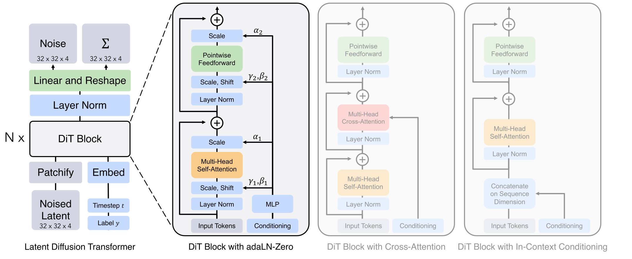
Diffusion 怎样进入压缩 latent 与 Transformer,见 Latent Diffusion、DiT 与 Flow;表示层的重建上限见 Autoencoder 与视觉 Tokenizer;控制条件如何注入与怎样公平评测见可控生成、编辑与评测。
加噪、prediction type 与 sampler 端点测试见多模态手撕实现。
Reference
- Hyvärinen, Estimation of Non-Normalized Statistical Models by Score Matching
- Vincent, A Connection Between Score Matching and Denoising Autoencoders
- Sohl-Dickstein et al., Deep Unsupervised Learning using Nonequilibrium Thermodynamics
- Song and Ermon, Generative Modeling by Estimating Gradients of the Data Distribution
- Ho et al., Denoising Diffusion Probabilistic Models
- Song et al., Denoising Diffusion Implicit Models
- Song et al., Score-Based Generative Modeling through Stochastic Differential Equations
- Nichol and Dhariwal, Improved Denoising Diffusion Probabilistic Models
- Dhariwal and Nichol, Diffusion Models Beat GANs on Image Synthesis
- Karras et al., Elucidating the Design Space of Diffusion-Based Generative Models
- Lu et al., DPM-Solver: A Fast ODE Solver for Diffusion Probabilistic Model Sampling in Around 10 Steps
- Ho and Salimans, Classifier-Free Diffusion Guidance